The food sector is a significant contributor to greenhouse gas emissions, contributing 10–32% of global anthropogenic sources. Compared with land-based food production systems, relatively little is known about the climate impact of seafood products. Previous studies have placed an emphasis on fishing activities, overlooking the contribution of the processing phase in the seafood supply chain. Furthermore, other studies have ignored short-lived climate forcing pollutants which can be particularly large for ship fuels. To address these critical knowledge gaps, we conducted a carbon footprint analysis of seafood products from Alaska pollock, one of the world’s largest fisheries. A holistic assessment was made including all components in the supply chain from fishing through retail display case, including a broad suite of climate forcing pollutants (well-mixed greenhouse gases, sulfur oxides, nitrogen oxides, black carbon and organic carbon), for domestic and top importers. We found that in some instances the processing phase contributed nearly twice the climate impact as the fishing phase of the seafood supply chain. For highly fuel-efficient fisheries, such as the Alaska pollock catcher-processor fleet, including the processing phase of the seafood supply chain is essential. Furthermore, the contribution from cooling emissions (sulfur and nitrogen oxides, and organic carbon) offsets a significant portion of the climate forcing from warming emissions. The estimates that include only greenhouse gases are as much as 2.6 times higher than the cases that include short-lived climate forcing pollutants. This study also advances our understanding of the climate impact of seafood distribution with products for the domestic retail market having a climate impact that is as much as 1.6 times higher than export products that undergo transoceanic shipping. A full accounting of the supply chain and of the impact of the pollutants emitted by food production systems is important for climate change mitigation strategies in the near-term.
Disclaimer: The findings and conclusions in the paper are those of the author(s) and do not necessarily represent the views of the National Marine Fisheries Service. Reference to trade names does not imply endorsement by the National Marine Fisheries Service, NOAA.
Introduction
The last decade has seen increasing interest in the climate impacts of food production (Vermeulen et al., 2012; Godfray et al., 2010; Foley et al., 2011). Among economic sectors, agriculture is one of the largest sources of greenhouse gas (GHG) emissions and accounts for 10–32% of global anthropogenic emissions (Heller and Keoleian, 2015; Eshel et al., 2014). Life cycle analysis studies reveal that consumer food choices can lead to a wide range of climate forcing (Heller and Keoleian, 2015; Hallström et al., 2015). Understanding the emissions associated with food is therefore critical for mitigating climate change and informing consumer behavior (Bajželj et al., 2014; Girod et al., 2014).
Globally, fisheries contribute ~4% of GHGs from the food sector (Parker et al., 2018). While this contribution is relatively small, seafood is a critically important source of nutrition (Parker et al., 2018). However, because environmental performance varies drastically between fisheries (Tyedmers, 2004; Schau et al., 2009; Parker et al., 2018), closer examination is needed in order to understand which fisheries contribute more or less to GHG emissions, and how they perform compared to other sources of protein (Tyedmers and Parker, 2012). While much has been learned about the emissions from land-based food sources, robust quantifications of seafood life cycle GHG emissions are relatively sparse (Nijdam et al., 2012; Clune et al., 2017). The limited information on seafood life cycle GHG emissions in part reflects the need for improved input data.
Previous studies have found that the life cycle GHG emissions are dominated by fuel combustion during fishing (Thrane, 2004; Guttormsdóttir, 2009; Svanes et al., 2011; Buchspies et al., 2011; Vázquez-Rowe et al., 2013), but the number of published studies is extremely small relative to the diversity of fishing methods and species targeted (Parker et al., 2015; Jafarzadeh et al., 2016). Given the limited number of studies and the assumption that fuel consumption is most important in the seafood supply chain, researchers may be overlooking the importance of processes downstream of fishing activities.
A further limitation of previous seafood emission studies is the focus on a narrow group of pollutants (e.g. well-mixed GHGs including CO2, CH4, and N2O) and the time horizon for the climate impact to occur (e.g. 100-y) (Tyedmers and Parker, 2012). Climate forcing over the coming decades will be strongly affected by short-lived climate forcing (SLCF) pollutants (Allen et al., 2018). SLCF pollutants, which include sulfur dioxide (SO2), nitrogen oxides (NOx), black carbon (BC), and organic carbon (OC), have short atmospheric lifespans and can have a strong warming (e.g. BC) or cooling (e.g. SO2, NOx, OC) effects on the earth’s energy budget. Although SLCF pollutants have been included in the estimation of cumulative emission budgets for ambitious mitigation goals (Allen et al., 2018), they have yet to be incorporated into the carbon footprints of food products.
While CO2 is the most important global GHG for most economic sectors, recent work revealed that the climate impact of the fishing activities can have large effects from pollutants other than CO2 (McKuin and Campbell, 2016). In particular, ignoring the cooling effects of SO2 can lead to overestimates in the climate forcing of fishing activities (McKuin and Campbell, 2016). However, that study did not investigate activities downstream of the fishing phase of the seafood supply chain. Thus, the impact of SLCF pollutants on processes downstream of fishing activities is largely unknown.
Given these challenges and the increasing importance of understanding seafood emissions, we conducted a carbon footprint analysis of the Alaska walleye pollock (hereafter, pollock) fishery in the eastern Bering Sea (EBS). The pollock fishery is globally important both in terms of volume and economic value of landings (Fissel et al., 2016). Over the past ten years, fillets and surimi have had roughly equal shares in the mass value of production of pollock products. The sustainability of the pollock fishery has been well studied within the context of fish stocks (Ianelli et al., 2017) and fisher responses to climate dynamics (Watson and Haynie, 2018), but very little study has been dedicated to the climate impact of fishing activities (Fulton, 2010). While the life cycle GHGs of white-fish (cod, haddock, and hake) fillet products has been studied (Ziegler and Hansson, 2003; Blonk et al., 2008; Guttormsdóttir, 2009; Sund, 2009; Winther et al., 2009; The Co-operative Group, 2010; Fulton, 2010; Iribarren et al., 2010; Sonesson et al., 2010; Buchspies et al., 2011; Svanes et al., 2011; Vázquez-Rowe et al., 2011; Vázquez-Rowe et al., 2012; Vázquez-Rowe et al., 2013), a peer-reviewed carbon footprint assessment of pollock products has not been conducted. Furthermore, the climate impact of shifts in production (e.g. processing and distribution) to different proportions of fillet and surimi market share are presently unknown.
To this end, we developed a first-order estimate of the climate forcing of primary pollock products, frozen battered-and-breaded fillets and crab-flavored sticks (e.g. imitation crab produced from pollock surimi) for the retail market on 20-y and 100-y time horizons. We included a 20-y time horizon because increasingly there are calls for the use of shorter time horizons to better reflect the climate change impacts of SLCF pollutants in the near-term (Myhre et al., 2013). We evaluated a broad range of climate forcing emissions (CO2, CH4, N2O, SO2, NOx, BC, and OC) and life cycle stages, including the fishing component through to the retail display case component of the product supply chain, for domestic and top importers of pollock fillet and surimi products. Furthermore, we evaluated the relative importance of these diverse life cycle stages and the potential to systematically assess the climate impact of alternative food sources.
Methods
Goal and scope
The aim of our study was to evaluate the comparative climate forcing per functional unit of 1 kg of frozen Alaska pollock product on two different time horizons (20-y and 100-y). The two products we surveyed include frozen battered-and-breaded fillets and frozen crab-flavored sticks for the top three markets. In the case of frozen battered-and-breaded fillets, we assume the products are produced from once-frozen fillet blocks and that the top three markets include Germany, the Netherlands, and domestic (United States) (Alaska Fisheries Science Center, 2016). In the case of frozen crab-flavored sticks, we assume the products are produced from once-frozen surimi blocks and the top three markets include Japan, South Korea, and domestic (United States) (Alaska Fisheries Science Center, 2016). We allocated the climate forcing impact among multiple products originating from the same process (e.g. fillets and fishmeal from fish processing) by mass value. The system boundaries of the production chain include fishing activities of catcher-processors up to the retail display case (Figure 1).

Overview of the seafood supply chain of pollock products for domestic and exported retail markets. (A): Supply chain of frozen battered-and breaded fillets for domestic (United States) and European retail markets. European retail markets are Germany and the Netherlands. (B): Supply chain of crab-flavored sticks for domestic and Southeast Asian retail markets. The Southeast Asian retail markets are Japan and South Korea. DOI: https://doi.org/10.1525/elementa.386.f1
Overview of the seafood supply chain of pollock products for domestic and exported retail markets. (A): Supply chain of frozen battered-and breaded fillets for domestic (United States) and European retail markets. European retail markets are Germany and the Netherlands. (B): Supply chain of crab-flavored sticks for domestic and Southeast Asian retail markets. The Southeast Asian retail markets are Japan and South Korea. DOI: https://doi.org/10.1525/elementa.386.f1
Life cycle inventory data collection
We compiled an inventory of materials and energy flows (inputs and outputs) of each phase of the seafood supply chain from technical reports and the literature.
In the fishing phase of the seafood supply chain, energy is consumed directly in the form of fuel used during fishing activities (Fissel et al., 2016) (Table S1). Materials and indirect energies (embodied in the materials) are consumed in the manufacture and maintenance of the fishing vessels and fishing gears (see Text S1.1 for detailed inputs). The material inputs include lubricating oil (Ziegler et al., 2015), cooling agent for air conditioning (Smith et al., 2014), metals (calculated using Equations S1-S3 and linear relationship between light ship weight and engine power given in Figure S1) (Fréon et al., 2014; Parker and Tyedmers, 2012), paints (anti-fouling paints and top-side paints calculated using Equations S4-S8) (Ziegler et al., 2015), and fishing gears (Table S2). To assist with the inventory analysis, we characterized the EBS catcher-processor fleet with respect to the number of active fishing vessels using data from the Alaska Commercial Fisheries Entry Commission (Table S3). We estimated the fuel quality for the fleet using the IHS Sea-web database, and vessel engine categories (Table S4). We obtained the annual catch of pollock and bycatch at the individual vessel-level from Pollock Conservation Cooperative and High Sea Catcher’s Cooperative reports (Table S5).
The primary processing phase of the seafood supply chain includes on-board production of intermediary products and storage of the product at a wholesaler (see Text S1.2 for detailed inputs). On-board the fishing vessel, energy is consumed directly in the form of fuel (used during processing of the fish on-board the fishing vessel) and electricity (for freezing the product). Material and indirect energy (embodied in the materials) is consumed in the manufacture of cooling agents for refrigerants (Smith et al., 2014) and the manufacture of packaging materials (Fulton, 2010). We obtained the annual production (2012–2015) of pollock products that were processed on-board the catcher-processor vessels from a NOAA National Marine Fisheries Service (NMFS) technical report (Table S6) (Fissel et al., 2016). During storage, energy (electricity for storing the frozen products) (Winther et al., 2009) is consumed directly and material and indirect energy are consumed in the manufacture of cooling agents for refrigerants (Bovea et al., 2007; Blowers and Lownsbury, 2010; Cascini et al., 2016; Winther et al., 2009).
We assumed two transportation modes, heavy-duty truck and container ship (see Text S1.3 for detailed inputs for transportation of intermediary products to secondary processors; see Text S1.4 for detailed inputs for transportation of final products to retail storage centers). The key inputs associated with both modes of transportation include fuel to power the main engines (and in the case of the container ship, the auxiliary engine) (Wang, 2011), container ship fuel for the temperature-controlled container freezer duty cycle (Fitzgerald et al., 2011), heavy-duty truck fuel for the temperature-controlled container freezer duty cycle (Tassou et al., 2009), and the coolant charge for temperature-controlled container for transport on the container ship (Smith et al., 2014) and on the heavy-duty truck (Tassou et al., 2009). We estimated the disposition of the product to each retail location by combining technical reports (Fissel et al., 2016) and trade data available from NMFS (Tables S7 and S8). We estimated the distances traveled by container ship (Table S9) and heavy-duty truck (Tables S10 and S11) using distance calculators and the literature (Text S1.3.3 and S1.4).
The secondary processing phase includes the energy and materials to produce the final product. In the case of frozen battered-and-breaded fillets, we used the inventory of materials and energy from a study that considered an identical product but a different white-fish (Patagonia grenadier) (Vázquez-Rowe et al., 2013). In the case of frozen crab-flavored sticks, we obtained the inventory of ingredients from the literature (Hur et al., 2011). We estimated the electricity demand for processing crab-flavored sticks by using published formulas for the energy demands of food processing (Sanjuán et al., 2014), and the rated power and loading rates in industry materials (Yanagiya Machinery Co., 2016).
In the retail activity phase of the seafood supply chain, electricity is consumed for freezer storage, for freezer and refrigerated display cases, and for ancillary operations (Tassou et al., 2011; Hoang et al., 2016; Winther et al., 2009). Materials and indirect energies (embodied in the materials consumed in the manufacture of coolants) (Bovea et al., 2007; Blowers and Lownsbury, 2010; Cascini et al., 2016) are consumed while the product is being stored at a retail distribution center, while the product is being stored at the retail store prior to display, and while it is on display at the retail store (see Text S1.5 for detailed inputs).
Carbon footprint data
We developed emission inventories by applying direct and indirect emission factors to the material and energy flows.
We applied direct emission factors to inventories of the fishing vessel, the container ship, and heavy-duty truck transport. We obtained emission factors for well-mixed GHGs (CO2, CH4 and N2O) and NOx of the fishing fleet and the container ship from a technical report (ICF International, 2009), from The Greenhouse Gases, Regulated Emissions, and Energy Use in Transportation (GREET) Model, Argonne National Lab v.1.3.0.12842 marine plug-in module, and from GREET’s Well-to-Wheel Vehicle Editor (Wang, 2011). We estimated BC emissions of the fishing fleet from plume sampling studies (Lack et al., 2008; Petzold et al., 2011; Buffaloe et al., 2014; Cappa et al., 2014). We calculated emissions of SO2 of the fishing fleet and container ship from the sulfur content in the fuel (Equation S9) (Faloona, 2009). We estimated the emissions of OC of the fishing fleet from the ratio of particulate organic matter to BC (Equation S10) (Petzold et al., 2011; Fuglestvedt et al., 2010) (see Text S2 for a detailed description of SLCF emission factors).
We applied indirect emission factors to inventories of materials and embodied energy used throughout the seafood supply chain. Following another study that included multiple food production stages, we used several existing tools to compile the life cycle inventory data (Xue and Landis, 2010). We developed indirect emission factors using life cycle assessment software including Simapro (v.7.2) and GREET, and the literature (see Tables S16 and S17 for detailed methods).
To consider the regional differences in energy sources for on-site electricity in the secondary processing and retail phases of the seafood supply chain, we developed separate electricity emission factors for each retail market. We applied emission factors to each energy source (obtained from GREET) to the energy mix of each country. We estimated the energy mix of each country using the fossil energy mix of each country (Energy Information Administration, 2018a) and an international energy statistics database (Energy Information Administration, 2018b).
Climate forcing calculations
To estimate the climate forcing of the two products, we applied a range of global warming potentials (GWPs) from the literature to the emission inventories of the seafood supply chain.
Metrics for individual land-based sectors are often similar to the global mean metric values (Shindell et al., 2008) while metrics for emissions from shipping show differences from global mean metric values (Myhre et al., 2013). These differences are largely due to the atmospheric chemistry in the environment into which ships emit pollutants. For example, due to the generally low-NOx concentration in the marine environment, the warming from ozone is outweighed by the stronger effect on CH4 destruction. Thus, the GWP of NOX for the shipping sector is lower than it is for land-based sectors. For this reason, we calculated the climate forcing of fishing and container ship activity with shipping GWPs (Eyring et al., 2007; Endresen et al., 2003; Fuglestvedt et al., 2008; Fuglestvedt et al., 2010; Collins et al., 2010; Myhre et al., 2013; Lauer et al., 2007; Aamaas et al., 2015) while for the other phases of the seafood supply chain we used a mean global metric GWP.
Because multiple products are produced from the Alaska pollock catcher-processor fleet, we used a mass balance approach to allocate impacts from the fishery and primary processing activities to each product. We normalized the climate forcing to the final products of each phase of the seafood supply chain (Equations S11–S17).
Uncertainty and sensitivity analysis
Carbon footprints come with large uncertainty in data and methods. Although we included standard deviations for certain parameters (fishing phase inputs, BC and OC emissions from the combustion of marine fuels, and shipping GWPs), we lack uncertainty measures for many of the downstream inputs of the seafood supply chain. Because we lack uncertainty data for downstream inputs, we did not consider stochastic variability. However, we did consider a sensitivity analysis to better understand which model inputs have the largest impact on the results and which factors contribute most to the output variability (Text S3). Our sensitivity analysis included material and energy flow inputs (Text S3.1), alternative emission factors (Text S3.2 and Tables 18 and 19), and alternative GWPs for shipping exhaust pollutants (Text S3.3).
Results
The results of the life cycle inventory, methods for emission factor estimates, emission factors, and GWPs for each phase of the seafood supply chain are presented in Tables 1, 2, 3, 4, 5, 6 and S12-S15, Tables S16-S19, Tables S20-S26, and Tables S27 and S28, respectively. The results of the sensitivity analysis input parameters are presented in Tables S29-S37.
Inventory of material and energy flows of the fishing phase of the seafood supply chain. DOI: https://doi.org/10.1525/elementa.386.t1
| Inventory item | Units | Amounta |
|---|---|---|
| Direct inputs | ||
| Fuel consumption in fishing operationsb,c,d | le | 6.88 (±0.88) × 107 |
| Marine lubricating oilf | kg | 2.07 (±0.13) × 105 |
| Refrigerant HFC-404a for air conditioningf | kg | 6.64 (±0.43) × 102 |
| Steel for vessel construction and maintenancef | kg | 4.56 (±0.30) × 106 |
| Copper wire for vessel construction and maintenancef | kg | 3.40 (±0.22) × 105 |
| Aluminum for vessel construction and maintenancef | kg | 2.47 (±0.16) × 105 |
| Cast iron for main engine constructiong | kg | 2.57 (±0.50) × 104 |
| Chrome steel for main engine constructiong | kg | 1.35 (±0.26) × 104 |
| Aluminum alloy for main engine constructiong | kg | 3.96 (±0.76) × 103 |
| Anti-fouling paintf | le | 8.79 (±0.57) × 102 |
| Primer paintf | le | 3.97 (±0.26) × 102 |
| Polyurethane paintf | le | 5.87 (±0.38) × 102 |
| Enamel paintf | le | 7.03 (±0.46) × 102 |
| Steel for fishing gearh | kg | 5.79 (±10) × 102 |
| Nylon for fishing gearh | kg | 7.73 (±0.13) × 102 |
| Lead for fishing gearh | kg | 5.02 (±0.09) × 103 |
| Polyethylene for fishing gearh | kg | 7.73 (±0.13) × 102 |
| Direct outputsi | ||
| Whole live-weight pollock | tj | 4.43 (±0.14) × 105 |
| Bycatch | tj | 3.99 (±1.23) × 104 |
a Mean and standard deviation in parenthesis.
b Product of the mean annual fuel consumption from American Fisheries Act (AFA) vessel survey results and the annual number of AFA catcher-processors participating in the fishery; 6 (±1)% of the total fuel consumption is allocated to processing.
c Errors (standard deviations) were propagated for the annual mean fuel consumption for fishing activities and the fraction of fuel consumption that is allocated to processing.
d Fuel type: 23% ultra-low sulfur diesel; 77% marine gas oil.
e Liters (l).
f The variation (standard deviation) is with respect to the number of AFA vessels.
g The error/variation (standard deviation) was propagated for the number of AFA vessels and the mass of main engines.
h The variation (standard deviation) is with respect to the AFA catch and the catch allocated to pollock.
i AFA annual catch (2012–2015) data obtained from the Pollock Conservation Cooperative and High Sea Catcher’s Cooperative Annual Reports (conf. Table S8).
j Metric tons.
Inventory of material and energy flows of the primary processing phase of the seafood supply chain. DOI: https://doi.org/10.1525/elementa.386.t2
| Inventory item | Units | Amounta |
|---|---|---|
| Direct inputs | ||
| Fuel consumption in on-board processingb,c,d | le | 4.39 (±0.53) × 106 |
| Refrigerantf for on-board freezingg | kg | 9.29 (±0.52) × 102 |
| Cardboardh | kg | 3.15 (±0.36) × 106 |
| Packaging film (LLDPE)h | kg | 3.62 (±0.42) × 104 |
| Liner (83% cardboard and 17% wax)h | kg | 2.07 (±0.24) × 106 |
| Initial chargei for freezer storage | kg | 4.30 (±0.50) × 102 |
| Refrigeranti leakage for freezer storageh | ||
| Energy consumption for freezer storageh | kJ | 2.86 (±0.33) × 1010 |
| Direct outputh,j | ||
| Whole fish | kg | 3.31 (±3.21) × 105 |
| Headed & gutted | kg | 2.24 (±0.45) × 107 |
| Roe | kg | 7.53 (±1.30) × 106 |
| Fillet | kg | 6.71 (±0.65) × 107 |
| Surimi | kg | 6.23 (±0.59) × 107 |
| Mince | kg | 1.60 (±0.19) × 107 |
| Meal | kg | 1.67 (±0.19) × 107 |
| Other | kg | 8.90 (±0.91) × 106 |
a Mean and standard deviation in parenthesis.
b Fuel consumption is the product of the mean fuel consumption in fishing operations (conf. Table 1) and the total fuel consumption allocated to processing (6 ± 1%) as reported in (Eyjólfsdóttir et al., 2003; Sund, 2009; Schau et al., 2009).
c Errors (standard deviations) were propagated for the annual mean fuel consumption for processing and the fraction of fuel consumption that is allocated to processing.
d Fuel type: 23% ultra-low sulfur diesel; 77% marine gas oil.
e Liters (l).
f R-134a.
g The variation (standard deviation) is with respect to the number of AFA vessels.
h The variation/error (standard deviation) was propagated for the BSAI at-sea pollock products, the AFA pollock catch, and the BSAI pollock retained catch by trawl catcher-processors.
i Ammonia.
j Mean values were computed as the product of the annual (2012–2015) Bering Sea & Aleutian Islands (BSAI) at-sea production of pollock products (conf. Table 14 in (Fissel et al., 2016)) and the ratio of the annual(2012–2015) pollock catch of the American Fisheries Act (AFA) catcher-processor fleet (conf. Table S5) to the BSAI annual (2012–2015) pollock retained catch by trawl catcher-processors (conf. Table 9 in (Fissel et al., 2016)).
Inventory of the secondary processing material and energy flows of frozen pollock battered-and-breaded filletsa. DOI: https://doi.org/10.1525/elementa.386.t3
| Item | Units | Amountb |
|---|---|---|
| Inputs | ||
| Frozen fillet blocks | kg | 6.71 (±0.65) × 107 |
| Packaging | kg | 1.76 (±0.17) × 106 |
| Reception | ||
| Lubricating oil (pallet jack and forklift) | kg | 4.61 (±0.25) × 102 |
| Electricity (pallet jack and forklift) | kWh | 1.35 (±0.13) × 104 |
| Unwrapping | ||
| Lubricating oil (forklift) | kg | 2.98 (±0.29) × 102 |
| Electricity (forklift) | kWh | 1.26 (±0.12) × 104 |
| Block cutting | ||
| Lubricating oil (band-saw) | kg | 2.94 (±0.28) × 102 |
| Electricity (band-saw) | kWh | 3.48 (±0.34) × 106 |
| Battering of fillets | ||
| Wheat-mix batter | kg | 8.45 (±0.81) × 106 |
| Tap water for battering process | kg | 1.96 (±0.19) × 107 |
| Electricity for mixing batter | kWh | 1.38 (±0.13) × 103 |
| Breadcrumb application | ||
| Breadcrumbs | kg | 2.94 (±0.28) × 107 |
| Electricity for coating machine | kWh | 6.94 (±0.67) × 102 |
| Industrial frying | ||
| Sunflower oil | kg | 4.23 (±0.41) × 106 |
| Electricity for oil sprinkler | kWh | 1.82 (±0.17) × 105 |
| Freezing | ||
| Electricity for freezing | kWh | 1.82 (±0.17) × 107 |
| Packaging | ||
| Cardboard | kg | 8.57 (±0.83) × 106 |
| Polyethylene | kg | 4.36 (±0.42) × 105 |
| Retractable polyolefin | kg | 6.16 (±0.59) × 105 |
| Electricity for packaging | kWh | 1.01 (±0.09) × 106 |
| Ancillary operations | ||
| Ammonia (NH3) | kg | 4.89 (±0.47) |
| Detergents | kg | 1.79 (±0.17) × 102 |
| Bleach | kg | 1.31 (±0.13) × 102 |
| Caustic soda | kg | 1.83 (±0.18) × 104 |
| Electricity | kWh | 4.86 (±0.47) × 107 |
| Outputs | ||
| Packaging for frozen fillet blocks | kg | 1.76 (±0.17) × 106 |
| Damaged fish blocks | kg | 6.04 (±0.58) × 106 |
| Fishsticks | kg | 1.21 (±0.12) × 108 |
| Fishstick packaging | kg | 9.62 (±0.93) × 106 |
| Excess breadcrumbs | kg | 1.84 (±0.16) × 106 |
| Excess batter | l | 1.60 (±0.15) × 103 |
a Inventory adapted from (Vázquez-Rowe et al., 2013).
b Mean and standard deviation in parenthesis. The varation/error (standard deviation) was propagated for the BSAI at-sea fillet, BSAI at-sea pollock products, the AFA pollock catch, and the BSAI pollock retained catch by trawl catcher-processors.
Inventory of secondary processing material and energy flows of frozen pollock crab-flavored sticksa. DOI: https://doi.org/10.1525/elementa.386.t4
| Item | Units | Amountb |
|---|---|---|
| Inputs | ||
| Frozen surimi blocks | kg | 6.23 (±0.59) × 107 |
| Packaging | kg | 1.63 (±0.15) × 106 |
| Reception | ||
| Lubricating oil (pallet jack and forklift) | kg | 4.48 (±0.42) × 102 |
| Electricity (pallet jack and forklift) | kWh | 1.31 (±0.12) × 104 |
| Unwrapping | ||
| Lubricating oil (forklift) | kg | 2.89 (±0.27) × 102 |
| Electricity (forklift) | kWh | 1.22 (±0.12) × 104 |
| Block cutting | ||
| Lubricating oil (band-saw) | kg | 2.86 (±0.27) × 102 |
| Electricity (band-saw) | kWh | 3.39 (±0.32) × 106 |
| Crab-flavored stick production | ||
| Electricity for kamaboko production | kWh | 9.43 (±0.89) × 106 |
| Wheat starch | kg | 3.12 (±0.29) × 106 |
| Potato starch | kg | 3.12 (±0.29) × 106 |
| Sugar | kg | 1.65 (±0.16) × 106 |
| Salt | kg | 1.52 (±0.14) × 106 |
| Crab extract | kg | 1.38 (±0.13) × 106 |
| Kelp extract | kg | 4.72 (±0.44) × 105 |
| Albumen | kg | 4.84 (±0.45) × 105 |
| Calcium carbonate | kg | 7.79 (±0.73) × 105 |
| Crab flavor | kg | 3.42 (±0.32) × 105 |
| Soybean oil | kg | 3.89 (±0.37) × 105 |
| Phosphate | kg | 2.36 (±0.22) × 105 |
| Seasoning mix | kg | 2.56 (±0.24) × 106 |
| Red colorant | kg | 3.54 (±0.33) × 104 |
| Distilled water | kg | 3.89 (±0.37) × 107 |
| Freezing | ||
| Electricity for freezing | kWh | 1.40 (±0.13) × 107 |
| Packaging | ||
| Cardboard | kg | 8.34 (±0.78) × 106 |
| Polyethylene | kg | 4.24 (±0.40) × 105 |
| Retractable polyolefin | kg | 5.98 (±0.56) × 105 |
| Electricity for packaging | kWh | 9.83 (±0.922) × 106 |
| Ancillary operations | ||
| Ammonia (NH3) | kg | 4.75 (±0.45) |
| Detergents | kg | 1.74 (±0.16) × 102 |
| Bleach | kg | 1.27 (±0.12) × 102 |
| Caustic soda | kg | 1.78 (±0.17) × 104 |
| Electricity | kWh | 4.72 (±0.44) × 107 |
| Outputs | ||
| Packaging for frozen surimi blocks | kg | 1.53 (±0.15) × 106 |
| Crab-flavored sticks | kg | 1.17 (±0.11) × 108 |
| Crab-flavored stick packaging | kg | 9.36 (±0.88) × 106 |
a Inventory adapted from (Hur et al., 2011).
b Mean and standard deviation in parenthesis. The varation/error (standard deviation) was propagated for the BSAI at-sea surimi, BSAI at-sea pollock products, the AFA pollock catch, and the BSAI pollock retained catch by trawl catcher-processors.
Inventory of the retail material and energy flows of frozen pollock products. DOI: https://doi.org/10.1525/elementa.386.t5
| Description | Units | Frozen battered-and-breaded filleta | Frozen crab-flavored sticka |
|---|---|---|---|
| Inputs | |||
| Product | kg | 1.21 (±0.12) × 108 | 1.17 (±0.11) × 108 |
| Packaging | kg | 9.62 (±0.93) × 106 | 9.36 (±0.88) × 106 |
| Retail distribution center | |||
| Electricity for freezer storageb | MJ | 2.41 (±0.23) × 106 | 2.34 (±0.20) × 106 |
| Coolant initial chargec | kg | 7.45 (±0.72) × 101 | 7.25 (±0.63) × 101 |
| Retail store | |||
| Electricity for freezer storaged | MJ | 3.44 (±0.33) × 106 | 3.35 (±0.29) × 106 |
| Leaked coolante | kg | 5.40 (±0.72) × 101 | 5.25 (±0.62) × 101 |
| Electricity for retail freezerd | MJ | 3.44 (±0.33) × 106 | 1.24(± 0.11) × 106 |
| Coolant initial chargee | kg | 1.05 (±0.21) × 102 | 1.02 (±0.15) × 102 |
| Electricity for ancillary operations | MJ | 1.97 (±019) × 107 | 1.07 (±0.17) × 107 |
| Outputs | |||
| Product | kg | 1.21 (±0.12) × 108 | 1.17 (±0.11) × 108 |
| Packaging | kg | 9.62 (±0.93) × 106 | 9.36 (±0.88) × 106 |
a Mean and standard deviation in parenthesis. The variation/error (standard deviation) was propagated for the BSAI at-sea surimi or fillets, BSAI at-sea pollock products, the AFA pollock catch, and the BSAI pollock retained catch by trawl catcher-processors.
b 7 days of storage time.
c Ammonia as coolant for retail distribution storage freezer.
d 10 days of storage time.
e Refrigerant R-404a as coolant for retail freezer (storage and display).
Literature values of the global warming potentials (GWPs) of various whitefish products. DOI: https://doi.org/10.1525/elementa.386.t6
| Product description | GWP-20y (kg CO2e kg product–1) | GWP-100y (kg CO2e kg product–1) |
|---|---|---|
| Frozen fillet products | ||
| Coda,b,c,d,e | 0.7–5.4 | |
| Saithec | 2.6 | |
| Haddockc | 3.7 | |
| Alaska pollockd | 1.1 | |
| Fresh fillet products | ||
| Codc,d | 2.4–2.6 | |
| Haddockf | 2.8–3.1 | |
| Hakeg | 7.3–11 | |
| Fresh gutted products | ||
| Codc | 3.6 | |
| Haddockc | 3.8 | |
| Miscellaneous products | ||
| Frozen cod, wetpackh | 2.2 | |
| Chilled cod loinsh | 4.4 | |
| Cod burgerg | 1.8 | |
| Salted codc | 2.2 | |
| “Clipfish” codc | 2.3 | |
| Landed hakei,j | 6.9–12 | |
| Alaska pollock crab-flavored stickk,l | 1.60 (±0.14)–1.81 (±0.18) | 1.47 (±0.13)–1.67 (±0.18) |
| Alaska pollock crab-flavored stickl,m | 0.92 (±0.20)–1.16 (±0.23) | 1.08 (±0.17)–1.29 (±0.20) |
| Product not specified | ||
| Codn,o | 3.4–4.8 | |
| Pollockn | 1.6 | |
| Frozen battered-and-breaded fillets | ||
| Codp | 3.4 | |
| Patagonian grenadierq | 2.2 | |
| Alaska pollockp | 1.2 | |
| Alaska pollockk,r | 1.85 (±0.17)–1.92 (±0.15) | 1.75 (±0.16)–1.78 (±0.14) |
| Alaska pollockm,r | 0.72 (±0.43)–1.16 (±0.21) | 1.08 (±0.17)–1.29 (±0.20) |
a (Ziegler and Hansson, 2003).
b (Guttormsdóttir, 2009).
c (Winther et al., 2009).
d (Fulton, 2010).
f (The Co-operative Group, 2010).
g (Vázquez-Rowe et al., 2011).
h (Svanes et al., 2011).
j (Vázquez-Rowe et al., 2012).
k This study, GHGs only.
l Range of values represents mean and standard deviations for U.S., South Korean, and Japanese retail markets.
m This study, baseline.
n (Blonk et al., 2008).
p (Sund, 2009).
q (Vázquez-Rowe et al., 2013).
r Range of values represents mean and standard deviations for U.S., Netherlands, and German retail markets.
Climate impact along the supply chain
Here, we present the climate impact results of two different Alaska pollock products (frozen battered-and-breaded fillets and crab-flavored sticks) for five different retail markets disaggregated by supply chain component (fishing, intermediary processing, transport to processor, secondary processing, transport to retail distribution centers, and retail activities) on 20-y and 100-y time horizons (Figure 2). We placed particular emphasis on a comparison of the processing contribution of the two seafood products (Figure 3).
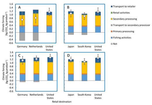
Mean climate impact of pollock products categorized by component in the seafood supply chain. The supply chain components include fishing activities, primary processing, transport to secondary processor, secondary processor, transport to retailer, and retail activities. Left panel (A, C): frozen battered-and-breaded fillets for three retail markets including Germany, the Netherlands, and the United States. Right panel (B, D): refrigerated crab-flavored sticks for three retail markets including Japan, South Korea, and the United States. Top panel (A, B): 20-y time horizon. Bottom panel (C, D): 100-y time horizon. The error bars represent standard deviations. DOI: https://doi.org/10.1525/elementa.386.f2
Mean climate impact of pollock products categorized by component in the seafood supply chain. The supply chain components include fishing activities, primary processing, transport to secondary processor, secondary processor, transport to retailer, and retail activities. Left panel (A, C): frozen battered-and-breaded fillets for three retail markets including Germany, the Netherlands, and the United States. Right panel (B, D): refrigerated crab-flavored sticks for three retail markets including Japan, South Korea, and the United States. Top panel (A, B): 20-y time horizon. Bottom panel (C, D): 100-y time horizon. The error bars represent standard deviations. DOI: https://doi.org/10.1525/elementa.386.f2

Mean climate impact of the secondary processing of pollock products categorized by activity. The processing activities include ancillary operations, packaging, product formation, block cutting, unwrapping, and reception. Left panel (A, C): frozen battered-and-breaded fillets for three retail markets including Germany, the Netherlands, and the United States. Right panel (B, D): refrigerated crab-flavored sticks for three retail markets: Japan, South Korea, and the United States. Top panel (A, B): 20-y time horizon. Bottom panel (C, D): 100-y time horizon. The error bars represent standard deviations. DOI: https://doi.org/10.1525/elementa.386.f3
Mean climate impact of the secondary processing of pollock products categorized by activity. The processing activities include ancillary operations, packaging, product formation, block cutting, unwrapping, and reception. Left panel (A, C): frozen battered-and-breaded fillets for three retail markets including Germany, the Netherlands, and the United States. Right panel (B, D): refrigerated crab-flavored sticks for three retail markets: Japan, South Korea, and the United States. Top panel (A, B): 20-y time horizon. Bottom panel (C, D): 100-y time horizon. The error bars represent standard deviations. DOI: https://doi.org/10.1525/elementa.386.f3
Across all time horizons and seafood products, the mean climate forcing (and standard deviations in parentheses) varies between 0.72 (±0.43)–1.32 (±0.17) kg CO2e kg product–1, in the case of battered-and-breaded fillets on a 20-y time horizon for the German retail market, and on a 100-y time horizon for the domestic retail market, respectively (Figure 2). Owing to the larger GWP potentials of the cooling SLCFs, the mean results on a 100-y time horizon are, remarkably, as much as 1.8 times higher than the estimates on a 20-y time horizon.
Examination of the results disaggregated by supply chain component indicate that, for several major pollock products, the downstream processing (transformation of primary products—frozen fillet blocks into frozen battered-and-breaded fillets or frozen surimi blocks into frozen crab-flavored sticks) can contribute more to the overall climate impact than the fishing phase (Figure 2). Across all products and time horizons, the mean (and standard deviation) climate forcing of the secondary processing phase of the seafood supply chain varies between 0.56 (±0.08)–0.66 (±0.09) kg CO2e kg product–1 (battered-and-breaded fillets for the German retail market on a 20-y time horizon and crab-flavored sticks for the Japanese market on a 100-y time horizon, respectively). The climate forcing for the fishing phase varies between 0.34 (±0.11)–0.35 (±0.17) kg CO2e kg product–1 (battered-and-breaded fillets on a 100-y time horizon and crab-flavored sticks on a 20-y time horizon, respectively). Thus, secondary processing contributes nearly twice the climate forcing as the fishing phase.
Given the importance of the processing stage in the pollock supply chain and the objective to compare the climate impact of processed surimi-type products with frozen fillet-type products, the climate forcing of the processing stage was examined in greater detail (Figure 3). Product formation (the embodied energy in product ingredients and electricity for production processes), packaging, and ancillary operations make almost equivalent contributions to the overall climate forcing associated with processing. For crab-flavored sticks, the mean (and standard deviation) climate forcing of product formation varies between 0.20 (±0.03)–0.24 (±0.03) kg CO2e kg product–1. Between 52–58% of the climate impact of product formation is attributed to product ingredients, with the remainder attributed to electricity consumption. For battered-and-breaded fillets, the mean (and standard deviation) climate forcing of product formation varies between 0.21 (±0.03)–0.23 (±0.03). In this case, 59–66% of the climate impact of product formation is attributed to product ingredients and the remainder is attributed to electricity consumption. Although the climate impact of electricity consumption is lower for battered-and-breaded fillets than for crab-flavored sticks, the ingredient burden is greater. This can be explained by the greater consumption of wheat ingredients for both batter and breading of the fillet product. As for the other processing activities, ancillary operations (electricity and embodied energy in the chemicals used by the processing facility such as bleach and detergents) and packaging, the climate impact is similar across products. The climate impact for ancillary operations varies between 0.17 (±0.03)–0.23 (±0.03) kg CO2e kg product–1. Packaging contributes between 0.17 (±0.02)–0.19 (±0.02) kg CO2e kg product–1.
Impact of including short-lived climate forcing pollutants
We evaluated the climate forcing of individual pollutants for pollock products for two scenarios and two different time horizons (Figures 4 and 5). The first scenario, hereafter referred to as the baseline, includes a large suite of pollutants including well-mixed GHGs and SLCFs. The second scenario includes only well-mixed GHGs (CO2, CH4, and N2O). We made comparisons at the chemical constituent level between the two products (battered-and-breaded fillets and crab-flavored sticks), between exported and domestic products, and between the two scenarios (Figures 4 and 5).
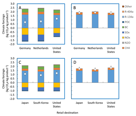
Mean climate forcing of pollock products by chemical constituent on a 20-y time horizon. Top panels (A, B): frozen battered-and-breaded fillets. Bottom panels (C, D): refrigerated crab-flavored sticks. Left panels (A, C): analysis including a suite of greenhouse gases (GHGs) and short-lived climate forcing pollutants. The category “other” is the combined impact of chlorofluorocarbons (CFCs 12 and 113) and hydrochlorofluorocarbon (HCFC 124). Right panels (B, D): analysis including only the three primary GHGs carbon (CO2, CH4, and N2O). The error bars represent standard deviations. DOI: https://doi.org/10.1525/elementa.386.f4
Mean climate forcing of pollock products by chemical constituent on a 20-y time horizon. Top panels (A, B): frozen battered-and-breaded fillets. Bottom panels (C, D): refrigerated crab-flavored sticks. Left panels (A, C): analysis including a suite of greenhouse gases (GHGs) and short-lived climate forcing pollutants. The category “other” is the combined impact of chlorofluorocarbons (CFCs 12 and 113) and hydrochlorofluorocarbon (HCFC 124). Right panels (B, D): analysis including only the three primary GHGs carbon (CO2, CH4, and N2O). The error bars represent standard deviations. DOI: https://doi.org/10.1525/elementa.386.f4

Mean climate forcing of pollock products by chemical constituent on a 100-y time horizon. Top panels (A, B): frozen battered-and-breaded fillets. Bottom panels (C, D): refrigerated crab-flavored sticks. Left panels (A, C): analysis including a suite of greenhouse gases (GHGs) and short-lived climate forcing pollutants. The category “other” is the combined impact of chlorofluorocarbons (CFCs 12 and 113) and hydrochlorofluorocarbon (HCFC 124). Right panels (B, D): analysis including only the three primary GHGs carbon (CO2, CH4, and N2O). The error bars represent the standard deviations. DOI: https://doi.org/10.1525/elementa.386.f5
Mean climate forcing of pollock products by chemical constituent on a 100-y time horizon. Top panels (A, B): frozen battered-and-breaded fillets. Bottom panels (C, D): refrigerated crab-flavored sticks. Left panels (A, C): analysis including a suite of greenhouse gases (GHGs) and short-lived climate forcing pollutants. The category “other” is the combined impact of chlorofluorocarbons (CFCs 12 and 113) and hydrochlorofluorocarbon (HCFC 124). Right panels (B, D): analysis including only the three primary GHGs carbon (CO2, CH4, and N2O). The error bars represent the standard deviations. DOI: https://doi.org/10.1525/elementa.386.f5
Climate forcing across the seafood supply chain by chemical constituent
Here, we evaluated the chemical constituents that contribute to warming and cooling across the seafood supply chain.
First, we examined the dominant chemical constituents of the two scenarios that contribute to warming. In the baseline scenario, warming is defined as the sum of the chemical constituents CO2, CH4, N2O, BC, CF4, C2F6, CF-12, CF-113, HCFC-124, R-134a, and R-404a. In the scenario that only considers GHGs, warming is defined as the sum of CO2, CH4, and N2O. CO2 is the dominant warming chemical constituent for all products and scenarios. The contribution from CO2 ranges from 1.38 to 1.72 kg CO2e kg product–1 for crab-flavored sticks for the South Korean market and battered-and-breaded fillets for the Netherlands market, respectively (Figures 4 and 5). However, other chemical constituents also have strong warming effects on the climate impact of the two seafood products. On a 20-y time horizon in the baseline scenario, BC is the second largest warming chemical constituent. In this case, BC contributes roughly 15% of the total warming, which varies between 2.00–2.47 kg CO2e kg product–1 (crab-flavored sticks for the South Korean market and battered-and-breaded fillets for the Netherlands market, respectively) (Figure 4A and 4C). On a 100-y time horizon in the baseline scenario, BC contributes roughly 5% of total warming species, which varies between 1.60–1.96 kg CO2e kg product–1 (crab-flavored sticks for the South Korean market and battered-and-breaded fillets for the Netherlands market, respectively) (Figure 5A and 5C). CH4 ranks second and third in order of importance for the scenario that considers only GHGs, and the baseline scenario, respectively. In the scenario that considers only GHGs on a 20-y time horizon, CH4 contributes roughly 13% of the total warming, varying between 1.60–1.92 kg CO2e kg product–1 (crab-flavored sticks for the South Korean market and battered-and-breaded fillets for the Netherlands market, respectively) (Figures 4B and 4D). In the scenario that considers only GHGs on a 100-y time horizon, CH4 contributes roughly 6% of the total warming, varying between 1.47–1.78 kg CO2e kg product–1 (crab-flavored sticks for the South Korean market and battered-and-breaded fillets for the Netherlands market, respectively) (Figure 5B and 5D). In the baseline scenario for both products, the contribution from CH4 to warming is between 10–12% and between 5–6% for the 20-y and 100-y time horizons, respectively (Figures 4A, 4C, 5A, and 5C).
Second, we examined the dominant chemical constituents of the baseline scenario that contribute to cooling on both time horizons and for both products. Here, cooling is defined as the sum of NOx, SOx, and OC. NOx is the dominant emission of the cooling chemical constituents on both time horizons and products (Figures 4A, 4C, 5A, and 5C). On a 20-y time horizon, the contribution of NOx varies between 50–56% of the mean total cooling emissions which varies between 1.05–1.66 kg CO2e kg product–1, for crab-flavored stick for the Japanese market and battered-and-breaded fillets for the German market, respectively. On a 100-y time horizon, the contribution of NOx varies between 71–76% of the mean total cooling species which varies between 0.52–0.77 kg CO2e kg product–1 for crab-flavored sticks for the Japanese market and battered-and-breaded fillets the German market, respectively. SOx is the next most dominant cooling chemical constituent for both time horizons and products (Figures 4A, 4C, 5A, and 5C). On a 20-y time horizon, the contribution of SOx varies between 35–43% of the mean total cooling species for crab-flavored sticks and battered-and-breaded fillets (all markets), respectively. On a 100-y time horizon, the contribution of SOx varies between 18–25% of the mean total cooling species for crab-flavored sticks and battered-and-breaded fillets (all markets), respectively.
SLCFs by individual components of the seafood supply chain
Here, we evaluated the dominant warming and cooling SLCFs by individual components of the seafood supply chain of the baseline scenario.
First, we considered an analysis of the individual components of the seafood supply chain activity at the chemical constituent level to identify where the dominant warming SLCF, BC, has the most significant impact. Disaggregated by individual processes, the fishing phase is the dominant source of BC emissions in the seafood supply chain across products and time horizons. On a 20-y time horizon for both products, the fishing phase contributes the vast majority of the mean total climate forcing of BC, contributing 76–88% of the total and varying between 0.32–0.38 kg CO2e kg product–1. On a 100-y time horizon for both products, the fishing phase contributes a similar 77–88% of the mean total climate forcing of BC which varies between 0.09–0.11 kg CO2e kg product–1. Transportation of product is second in order of impact of the mean total climate forcing of BC emissions. In the case of products for non-domestic markets on both time horizons, the transportation of products to secondary processors phase of the seafood supply chain contributes 3–4% of the BC climate forcing. In the case of products for the domestic market on both time horizons, the transportation of products to retailer phase of the seafood supply chain contributes roughly 5% of the BC climate forcing.
Second, we considered the contribution of the primary cooling SLCF constituent, NOx, by supply chain activity. In this case, fishing makes an important contribution to the overall source of the mean total climate forcing of NOx. In the case of battered-battered-and-breaded fillets for European markets on a 20-y time horizon, fishing contributes roughly 63% of the NOx cooling value of 0.82 kg CO2e kg product–1. In the case of the other markets and products on a 20-y time horizon, fishing contributes roughly 85% of the NOx cooling value of 0.60 kg CO2e kg product–1. In the case of battered-and-breaded fillets for European markets on a 100-y time horizon, fishing contributes roughly 60% of the NOx cooling value of 0.54 kg CO2e kg product–1. In the case of the other markets and products on a 100-y time horizon, fishing contributes roughly 80% of the NOx cooling value of 0.40 kg CO2e kg product–1. Transportation of products is the second largest source of NOx emissions. In the case of products for non-domestic markets on both time horizons, the transportation of products to secondary processors contributes roughly 34% of the NOx climate forcing for both products. In the case of products for the domestic market on both time horizons, the transportation of products to retailers contributes roughly 12% of the NOx climate forcing for both products.
Comparisons between retail markets
Here, we compared our climate forcing estimates of pollock products for the domestic (United States) market to pollock products for foreign markets (Germany, the Netherlands, Japan, and South Korea).
Comparing estimates in the baseline scenario reveals that the climate impact of exported products is generally lower than domestic products. On a 20-y time horizon, the climate forcing of products for the domestic market is between 1.1–1.6 times higher than products for foreign markets. On a 100-y time horizon, the climate forcing of products for the domestic market is between 1.1–1.2 times higher for foreign markets. This can be explained by the fact that exported products undergo transoceanic shipping, which results in higher amounts of cooling species than the domestic products. Although domestic products are also shipped by container ship, roughly 40% of the short shipping route (from Port of Dutch Harbor to Port of Seattle) takes place within emission control areas where the sulfur in marine fuels is regulated (0.1% wt. sulfur in fuel). The exported products, on the other hand, travel greater distances in regions outside of emission control areas (in the case of the products shipped to Southeast Asian markets, the entirety of the route is outside emission control areas) where the sulfur in marine fuels is an order of magnitude higher (global average is ~2.4% wt. sulfur in fuel). There is also variability in net climate forcing between domestic and export retail markets due to the differences in energy sources for grid electricity (Figure S2).
For battered-and-breaded fillets in the scenario that only includes GHGs, the climate impact of product for the German and domestic market is very similar regardless of the retail distribution location or time horizon (Figures 4B and 5B). The first explanation is that although the product for the German retail market travels a greater overall distance, the product shipped by container ship is in an unfinished form with a smaller shipping mass. The domestic product is shipped a shorter distance but in a finished product form and thus with a greater shipping mass. Second, we assume that domestic products travel a greater distance to the retail markets than the exported products. Unlike battered-and-breaded fillets, the climate impact of the exported and domestic crab-flavored sticks has similar trends in both the baseline scenario and the scenario that only considers GHGs (Figures 4C, 4D, 5C, and 5D).
Comparisons between scenarios
Here, we compared the climate impact of the baseline cases to the climate impact of the scenario that considers only GHGs (Figures 4 and 5). For battered-and-breaded fillets on a 20-y time horizon, the climate impact of the scenario considering only GHGs varies between 1.85 (±0.17)–1.92 (±0.15) kg CO2e kg product–1 (Figure 4B). In this case, the climate forcing is between 1.6–2.6 times higher than the baseline scenarios (Figure 4A and 4B). On a 100-y time horizon, the climate impact of battered-and-breaded fillets considering only GHGs varies between 1.75 (±0.16)–1.78 (±0.14) kg CO2e kg product–1 (Figure 5B). In this case, the climate forcing is between 1.3–1.5 times higher than the baseline (Figure 5A and 5B). For crab-flavored sticks on a 20-y time horizon, the climate impact of the scenario considering only GHGs varies between 1.60 (±0.14)–1.81 (±0.18) kg CO2e kg product–1 (Figure 4D). In this case, the climate forcing is between 1.6–1.7 higher than the baseline scenario (Figure 4C and 4D). On a 100-y time horizon, the climate impact of crab-flavored sticks considering only GHGs varies between 1.47 (±0.13)–1.69 (±0.17) kg CO2e kg product–1 (Figure 5D). In this case, the climate forcing is between 1.3–1.4 times higher than the baseline scenario (Figure 5C and 5D).
Sensitivity Analysis
We conducted a sensitivity analysis of each phase of the seafood supply chain (extended results are provided in Text S4.1-S4.6 and Figures S3-S14). Here, we consider separately the key results of the secondary processing and the sum total of the seafood supply chain. For the sum total of the seafood supply chain, we considered the parameters that contributed most to the variance in the standard deviations, and the impact of alternate parameters that are highly uncertain but not included in the standard deviations.
Although we did not find a substantial difference between the secondary processing climate impact of crab-flavored sticks and battered-and-breaded fillets in our baseline assessment, we did find a modest difference between the two products when we applied alternate emission factors in the sensitivity analysis. We found an increase of 26% and 19% in the climate forcing of breaded-and-battered fillets over crab-flavored sticks on 20-y and 100-y time horizons, respectively (Text S4.4.2).
In the case of sum total of the seafood supply chain across products and time horizons, the top contributors to the variance in the standard deviations were the mass of the intermediary product (frozen surimi or frozen fillets), and the shipping GWPs of SLCF pollutants (NOx, SOx, BC, and OC) (Text S4.7.1 and Figure S13).
In the case of highly uncertain variables for the sum total of the seafood supply chain, the parameters that have the largest impact on the net climate forcing values depend on the product, the market, and the time horizon (Text S4.7.2 and Figure S14). In all cases (products, markets, and time horizons), using the global mean metric GWP instead of the shipping GWP for the shipping exhaust emissions, had the largest impact. On a 20-y time horizon, the global mean metric GWPs of SLCFs have differences between 4.5–124% (in the case of BC and NOx, respectively) compared with the shipping GWPs for SLCFs. As a result of the using the global mean metric GWP instead of the shipping GWP for shipping exhaust SLCFs, the climate forcing of the products increased by over 2.5 times the baseline results for the European market (Germany and Netherlands), and increased by nearly double the baseline results for all other markets. On a 100-y time horizon, the global mean metric GWPs of SLCFs have differences between 1.4–74% (in the case of BC and NOx, respectively) compared with the shipping GWPs for SLCFs. As a result of using the global mean metric GWP instead of the shipping GWP for shipping exhaust SLCFs, the climate forcing of products varied between 24–38% above the baseline results. Reducing the sulfur level in marine fuel to 0.5 (% wt.) was second in order of impact for battered-and-breaded fillets to European markets on a 20-y time horizon. In this case, reducing the sulfur level in marine fuels by 86% from the mean value of 2.4 (% wt.), resulted in increases in net climate forcing of 1.5 times above the baseline values. In all other cases, the distances traveled by heavy-duty trucks was second in order of impact. Decreases in distances between 67–83% resulted in decreases in net climate forcing results between 6–22% below the baseline values for all markets. Increases in distances between 55–559% resulted in increases in net climate forcing between 8–28% above baseline values for foreign markets (increase in distance was negligible for products for the domestic market). The variance in the sulfur levels in fuel was third in order of impact for battered-and-breaded fillets to European markets on a 20-y time horizon. Adjusting the sulfur level in marine fuels by ±46% resulted in differences in net climate forcing of ±30% from the baseline values. In all other cases, the number of days the products spend in storage was third in order of impact. Adjustments of ±49% in storage time over the entire seafood supply chain resulted in changes in net climate forcing between ±8–15% from baseline values.
Discussion
Here, we discuss the results of our processing inputs—which are between 1.6–1.9 times higher than the fishing inputs—and our net baseline results (including SLCF pollutants)—which are between 1.3–2.6 times higher than the results with GHGs only—from the perspective of the limitations of this study. Additionally, we compare this study to other research.
We compared the results of our study to life cycle assessment and carbon footprint studies of white-fish (e.g. cod, hake, and pollock) (Table 6). Although direct comparisons are difficult to make due to differences in fish species, fishing methods, product forms, system boundaries, the chemical constituents included, and allocation methods—the results of this study fall within the wide range of literature values (0.70–14.2 kg CO2e kg white-fish product–1). The studies that are more comparable to this research include those with pollock products (Blonk et al., 2008; Sund, 2009; Fulton, 2010) and the studies of breaded white-fish products (Sund, 2009; Vázquez-Rowe et al., 2013). Our results are in agreement with the GWP of pollock products found in other studies, which vary between 1.1–1.6 kg CO2e kg product–1. In the case of breaded white-fish fillets, the GWPs found in other studies vary between 1.2–3.4 kg CO2e kg product–1. Our climate forcing estimates of frozen battered-and-breaded fillets on a 100-y time horizon are as much as 1.1 times the GWP estimate of breaded Alaska pollock fillets, and between 34–39% of the estimate of the breaded cod fillets reported by Sund (2009). A lack of detail related to the processing material and energy flows in Sund (2009) however, make it difficult to explain the reason for the differences between studies. The GWP of breaded Patagonian grenadier fillet product reported by Vázquez-Rowe et al. (2013) is between 1.7–1.9 times higher than our estimates of battered-and-breaded Alaska pollock fillets on a 100-y time horizon.
Owing to the fact that the material and energy flows for the processing of frozen Alaska pollock fillet blocks for this study were adapted from Vázquez-Rowe et al. (2013), a more detailed comparison between studies may be warranted. Despite the smaller system boundary of Vázquez-Rowe et al. (2013) (which includes the seafood supply chain components up to the production facility gate) the fishing phase makes up approximately 70% of the total climate burden, and processing and ingredients make up the remainder. In this study, however, processing makes up the larger share of the climate burden with fishing activities contributing roughly 30% in the baseline case on a 100-y time horizon. The higher apportionment of the climate burden to the processing phase and lower apportionment of the climate burden to the fishing phase in the seafood supply chain can be explained by the higher fuel efficiency of the Alaska pollock fleet. The fuel consumption of the Alaska pollock fleet, 152 (±36) liters of fuel metric ton (mt) fish–1, is only 32% of the fuel consumption of the Patagonian grenadier fleet, 469 liter of fuel mt fish–1. Second, unlike Vázquez-Rowe et al. (2013), our study did not include the co-products of fish feed from broken fillet blocks. Furthermore, other important co-products for Alaska pollock processing may include fish oil that could be used to offset the fuel for fishing and/or production (Yuvaraj et al., 2016).
We did not find a significant difference between the climate impact of crab-flavored sticks and battered-and-breaded fillets in our baseline assessment. However, before drawing inferences it is important to point out study limitations. First, the choice of database and software program for the emission factors is an important consideration that may add uncertainty to the results. Our sensitivity analysis of the processing inputs found modest increases in the climate forcing of breaded-and-battered fillets over crab-flavored sticks when we used alternative emission factors for the ingredient inputs. It has been pointed out that quantitative uncertainty in life cycle inventory data, characterization factors and methodological choices are necessary for robust statistical confidence (Henriksson et al., 2015). Future studies should include uncertainties of the emission factors for all phases of the seafood supply chain. Second, we did not include quantitative uncertainty with respect to downstream phases of the products (e.g. processing of the fish into battered-and-breaded fillets and crab-flavored sticks) because the data we relied on to develop those inventories did not report uncertainties (Vazquez-Rowe et al., 2013; Hur et al., 2011). As more data becomes available, future studies should consider uncertainties of the downstream processing phases of the products. Third, our inputs of the processing phase for crab-flavored sticks were hypothetical. We relied on values from the literature for the ingredients, and used rated power and loading rates found in industry materials. On the other hand, while our inputs for the battered-and-breaded fillets also relied on a detailed inventory from the literature, that study obtained the data directly from an industrial plant. Thus, our study of crab-flavored sticks could be improved by obtaining more detailed inventory data from industrial processors.
The uncertainty in our climate forcing results for the battered-and-breaded fillets on a 20-y time horizon are on the order of 34% and 59% for the Netherlands and German markets, respectively. As pointed to in our sensitivity analysis of variables included in the standard deviations, the variability in the mass of the fillets to these markets over a 4-year period and the variability in the shipping SLCF GWPs are the key uncertainty drivers. Future studies should consider longer-term trends and perform statistical analyses for robust confidence intervals.
Our climate impact study used an attributional life cycle approach, and did not consider the broader environmental and economic interactions of a consequential approach. Recently, it was found that environmental interactions (such as pollock abundance and water temperature) are important drivers in Alaska pollock catcher-vessel operational decisions such as choice of fishing location and trip length (Watson and Haynie, 2018). In that study, economic interactions were also found to be important because the strategies fishers used to deal with environmental variables were different depending on whether the vessels were catching fish to produce surimi or fillets. These observations have implications for our study because fuel usage from the fishing phase varies with environmental conditions and fish stocks, and the actual production composition (and subsequent downstream impacts) may vary inter-annually when the relative amounts of surimi and fillet products fluctuate. We considered the inputs of a subset of the catcher-processor fleet which in 2018 represented roughly 40% of the total Alaska pollock catch in the U.S. To have a more complete understanding of the sustainability of Alaska pollock, future studies should consider the climate impact of the catcher-vessel fleet in the Bering Sea and Gulf of Alaska and incorporate important environmental and economic interactions that occur from year to year.
We assumed that the majority of the products from the catcher-processor fleet follow the once-frozen fillet production supply chain (Alaska Fisheries Science Center, 2016). However, a significant portion of headed and gutted pollock production is exported to China for twice-frozen fillet production (Alaska Fisheries Science Center, 2016). In this case, the headed and gutted pollock is processed into frozen fillet blocks in China, then reimported to the domestic or European processors. Given the large impact that transoceanic shipping has on the climate impact of these products, future studies should consider the supply chain of pollock that is landed in the United States that is exported for processing and shipped back into the United States. This may prove difficult, however, because increasingly globalized seafood supply chains complicate efforts to track a single product and its sustainability (Gephart et al. 2019). Thus, improved estimates of the climate impact of U.S. pollock products will require greater transparency from industry actors throughout the supply chain.
Conclusions
First, this study contributes to the food-miles debate (Weber and Matthews, 2008; Coley et al., 2009; Yang and Campbell, 2017) given the findings that ship transportation inputs play a large role in the climate forcing of pollock products. In particular, the effect of using shipping GWPs instead of the global mean metric GWPs for the SLCF exhaust emissions from ships had the largest impact on the results over the entire seafood supply chain. Furthermore, for products that undergo transoceanic shipment by container ship, the cooling from sulfur oxides resulting from the combustion of marine fuels have a substantial effect on the climate impact of pollock products. Considering the large effect from sulfur oxides, there may be important policy implications for the future climate impact of seafood. The current maximum sulfur content of marine fuels of 3.5%, set by the International Maritime Organization’s Marine Environmental Protection Committee, will be reduced to a maximum of 0.5% by 2020 (Smith et al., 2014). As a result of this policy, the cooling effect of sulfur oxides may be diminished and there may be a near-term increase in the future climate impact of all food that is shipped on transoceanic voyages. Thus, the reduction in sulfur content could lead to a significant increase in climate forcing. However, the climate impact should be weighed against the human health (e.g. reduced particulate matter emissions) and environmental benefits (e.g. reduced acidification potential) of reduced sulfur contents in marine fuels (Hassellöv et al., 2013; Sofiev et al., 2018).
Second, we found that on average the climate impact of the downstream processes was nearly twice that of the fishing phase of the seafood supply chain. These results can provide benchmarks for comparisons and the identification of processing of intermediary products as a “hot-spot” can help industry actors understand where to concentrate their carbon footprint reduction efforts. We emphasize, however, that the finding that climate impact from processing outweigh those of fishing may not apply to all seafood products, but are more relevant for highly fuel-efficient fisheries. Nevertheless, our results do illustrate the need for comprehensive carbon footprints across the entire supply chain.
Lastly, we found the climate impact of the products in the scenario that includes only GHGs is as much as 2.6 times higher than the products that include SLCFs in the analysis. There is a growing consensus among policy-makers and scientists that efforts to address climate change should not be limited to reductions of CO2 but should be complemented by mitigation of SLCFs in the near-term (Smith and Mizrahi, 2013; Rogelj et al., 2014). Thus, an improved accounting of the climate impact of food production systems should also consider the contribution of SLCFs.
Data Accessibility Statement
The datasets used to construct indirect emission factors of non-ingredient materials and fuels (Table S24), indirect emission factors of ingredients (Table S25), alternative indirect emission factors of non-ingredient materials and fuels used in the sensitivity analysis (Table S35), and alternative indirect emission factors of ingredients used in the sensitivity analysis (Table S36) are available at https://doi.org/10.6071/M3HW93.
Acknowledgments
We gratefully acknowledge helpful feedback on a previous version of this manuscript from M. Beman, G. Villalba, and M. Beutel.
Funding information
BLM was supported by a UC Merced, Environmental Systems Summer Fellowship.
Competing interests
The authors have no competing interests to declare.
Author contributions
Contributed to conception and design: BLM, JTW, ACH, JEC
Contributed to acquisition of data: BLM
Contributed to analysis and interpretation of data: BLM, JTW
Drafted and/or revised the article: BLM, JTW, ACH, JEC
Approved the submitted version for publication: BLM, JTW, ACH, JEC