This paper presents the first empirical estimates of dimethyl sulfide (DMS) gas fluxes across permeable sea ice in the Arctic. DMS is known to act as a major potential source of aerosols that strongly influence the Earth’s radiative balance in remote marine regions during the ice-free season. Results from a sampling campaign, undertaken in 2015 between June 2 and June 28 in the ice-covered Western Baffin Bay, revealed the presence of high algal biomass in the bottom 0.1-m section of sea ice (21 to 380 µg Chl a L–1) combined with the presence of high DMS concentrations (212–840 nmol L–1). While ice algae acted as local sources of DMS in bottom sea ice, thermohaline changes within the brine network, from gravity drainage to vertical stabilization, exerted strong control on the distribution of DMS within the interior of the ice. We estimated both the mean DMS molecular diffusion coefficient in brine (5.2 × 10⁻⁵ cm2 s–1 ± 51% relative S.D., n = 10) and the mean bulk transport coefficient within sea ice (33 × 10–5 cm2 s–1 ± 41% relative S.D., n = 10). The estimated DMS fluxes ± S.D. from the bottom ice to the atmosphere ranged between 0.47 ± 0.08 µmol m–2 d–1 (n = 5, diffusion) and 0.40 ± 0.15 µmol m–2 d–1 (n = 5, bulk transport) during the vertically stable phase. These fluxes fall within the lower range of direct summer sea-to-air DMS fluxes reported in the Arctic. Our results indicate that upward transport of DMS, from the algal-rich bottom of first-year sea ice through the permeable sea ice, may represent an important pathway for this biogenic gas toward the atmosphere in ice-covered oceans in spring and summer.
Introduction
Dimethyl sulfide (DMS) is the most abundant gaseous precursor of atmospheric sulfate aerosols in remote marine regions (Bates et al., 1992; Andreae and Crutzen, 1997). Aerosols strongly influence the Earth’s radiative balance, either via direct scattering of solar radiations back to space, or indirectly by acting as condensation nuclei upon which clouds may form and grow (Curran and Jones, 2000). Pristine atmospheric conditions that may be found at high latitudes (Vogt and Liss, 2009) make DMS-derived aerosols significant in regional cloud formation processes (Carslaw et al., 2013).
DMS production arises mostly from the degradation of the ubiquitous phytoplankton osmolyte dimethyl sulfoniopropionate (DMSP) produced by several phytoplankton species (e.g., Green and Hatton, 2014). DMSP plays various roles in phytoplankton, including osmoregulation (Kirst et al., 1991; Lyon et al., 2016), cryoprotection (Karsten et al., 1996), and prevention of cellular oxidation (Sunda et al., 2002). DMSP-to-DMS conversion is mediated by DMSP-lyases, enzymes that are found in bacteria and a few microalgal groups including Haptophyceae and Dinophyceae (Niki et al., 2000). DMS is also linked to dimethyl sulfoxide (DMSO), a cellular metabolite that is both a source and a sink of DMS through oxidation and bacterial consumption processes, respectively (Asher et al., 2011; Hatton et al., 2012). The two other major sinks of DMS in the marine environment are photo-oxidation and ventilation (Brimblecombe and Shooter, 1986). Ultimately, between 18 and 34 Tg of S y–1 are ventilated as DMS, making this gas the main contributor to the global biogenic flux of atmospheric sulfur (Lana et al., 2011).
Sea ice is a major player in biogeochemical cycles, including the cycling of sulfur (Tison et al., 2010). In the Arctic, most of the algal biomass in spring concentrates in the lowermost part of the ice (Smith et al., 1990; Juhl et al., 2011; Galindo et al., 2014). Ice algae in the bottom sea ice benefit from a renewed supply of nutrient-rich under-ice water, relatively stable temperatures and a substrate that prevents the cells from sinking and allows them to harvest the available light below the snow and ice covers (Horner et al., 1992). Arctic ice-algal blooms are associated with extremely high levels of DMSP (Levasseur et al., 1994; Galindo et al., 2014) and DMS (Carnat, 2014). In the Antarctic too, the exceptionally high algal biomass typically encountered at the bottom of sea ice is generally associated with concentrations of DMS that are 2 to 3 orders of magnitude higher than those measured in under-ice water (Turner et al., 1995; Gambaro et al., 2004; Carnat et al., 2014).
Still, most climatology-derived estimates consider that DMS fluxes above ice-covered waters are negligible, typically because of the paucity of sea ice-related data (Lana et al., 2011). The quantification of gas in sea ice is indeed technically challenging, and measurements of gas fluxes at the ice-atmosphere interface are notoriously difficult to achieve (Vancoppenolle et al., 2013; Tison et al., 2017). However, recent studies have shown that sea ice, through its liquid brine and air bubble-filled porosity, can exchange gases with both the ocean and the atmosphere (Fanning and Torres, 1991; Loose et al., 2011; Trevena and Jones, 2012). The amount, size and shape of the brine inclusions govern the permeability of ice to fluid and gas transport (Golden et al., 1998; Loose et al., 2009). Seasonal sea ice warming increases the size and connectivity of brine channels. This raises the ice permeability and consequently, the potential transport of DMS within the ice cover (Tison et al., 2017). DMS fluxes varying between 0.2 and ca. 30 µmol m–2 d–1 have been measured directly and indirectly over Antarctic sea ice (Zemmelink et al., 2008; Nomura et al., 2012; Trevena and Jones, 2012; Carnat et al., 2014), but to our knowledge, empirical measurements of DMS fluxes above the Arctic sea ice have not been reported. Convection, diffusion, and bubble nucleation and migration through buoyancy together control gas transport within permeable sea ice (Zhou et al., 2013; Crabeck et al., 2014, 2019). These gas transport processes may play a role in the fate of the high DMS concentrations produced during ice-algal blooms in the Arctic.
This study aimed to provide the first empirical estimations of upward DMS transport through the ice and potentially to the atmosphere in the Arctic. We conducted a suite of DMS measurements in sea ice and ice-associated environments (melt ponds, snow, under-ice water), which provided a broad picture of the different ice-related sources of DMS in the sampling region. These measurements were combined with a thorough analysis of the changes in the sea-ice thermohaline regime during the melt period, allowing us to highlight physical processes involved in DMS distribution within the internal ice layers and to estimate DMS fluxes and transport coefficients (DDMS). We investigated both dissolved DMS diffusion and gaseous transport of DMS (bubbles) as potential pathways for DMS across permeable first-year sea ice (FYI).
Materials and methods
Study area and sampling
Sampling operations took place within a 500-m radius around an ice camp (67.28°N; 63.47°W) located southeast of the Qikiqtarjuaq hamlet (Nunavut), near Baffin Bay (Figure 1). Sampling was conducted in 2015 from June 2 to 28, with samples collected every two days from June 2 to June 12 and every three days from June 15 to 28. Nine full profiles of sea ice were collected, coupled with measurements of the overlying snow cover at four stations, seven under-ice water (0.5 m below sea ice) samplings, and three melt ponds. This effort was part of the Green Edge project, a multidisciplinary project aiming to understand the key physical, chemical and biological processes governing the spring algal blooms in the Arctic Ocean.

Map of the sampling region and location of the Green Edge 2015 ice camp. Red circle indicates position of the ice camp (67° 28′ N, 63° 47′ W). DOI: https://doi.org/10.1525/elementa.370.f1
Map of the sampling region and location of the Green Edge 2015 ice camp. Red circle indicates position of the ice camp (67° 28′ N, 63° 47′ W). DOI: https://doi.org/10.1525/elementa.370.f1
Environmental measurements
Air temperature was monitored every 10 minutes using an automated meteorological tower (HC2S3, Campbell Scientific®) (67.28°N; 63.47°W). Upon arrival on site, snow depth was measured with a metal ruler at five to eight randomly selected locations around the sampling site. Snow profiles were also collected for DMS and salinity measurements using Whirl-pack® bags (300 mL) in which excess air surrounding the sample was removed using a manual pump. Melted snow salinity was determined using a conductivity probe (Cond 330i, WTW conductivity probe; precision of ±0.1%).
Ice cores were collected using a 0.09-m core barrel (Kovacs Mark II) in order to obtain physical measurements on the sea ice. Sea-ice depth and freeboard, the height of sea ice above the ocean surface, were measured through the ice core holes using a thickness gauge (Kovacs Enterprise). In situ sea-ice temperature and bulk salinity profiles were measured following Miller et al. (2015). Sea-ice temperature profiles were measured directly in one dedicated ice core at 0.1-m intervals using a high-precision thermometer (Testo 720; ±0.1°C). The ice core was then cut into 0.1-m slices using a handsaw, and the slices were stored in a plastic container and melted at room temperature. Bulk salinity of the melted ice sections was determined using a conductivity probe, as described above.
Once melt ponds formed on the sampling site (after June 23), melt-pond depth, length and width were determined using a graduated stick and tape ruler. Melt-pond water temperature and salinity were measured using a high-precision thermometer (61220-601 digital data logger, VWR) and a conductivity probe (Cond 330i, WTW conductivity probe; precision of ±0.1%), respectively.
Physical properties of sea ice
Brine volume fraction (Vbr), a proxy of sea-ice permeability, was calculated from sea-ice bulk salinity and in situ temperature measurements using the parameterization of Leppäranta and Manninen (1988) for sea-ice temperatures >–2°C, and that of Petrich and Eicken (2010) for sea-ice temperatures <–2°C. Brine inclusions are expected to become interconnected when Vbr reaches 5% for columnar sea ice (Golden et al., 2007). Gas bubble transport across the brine system has been reported to occur when Vbr reaches 7.5–10% (Zhou et al., 2013).
Brine salinity (Sbr) was calculated using the formulation of Notz (2005):
where T is the ice temperature in degrees Celsius.
The Rayleigh number (Ra, dimensionless) was calculated to assess the propensity of brine gravity drainage within the sea-ice cover (Equation 2). Ra is currently used as an indicator of the onset and strength of gravity drainage during ice growth in polar regions (Notz and Worster, 2009) and has also been used to describe the dynamics of sea ice during spring melt (e.g., Carnat et al., 2013):
where g = 9.81 m s–2 is the acceleration due to gravity; β(Sbr(z) – Suiw) is the density difference (kg m–3) across a vertical distance Δz between seawater and brine at depth z (m) (Δz = 0 at the ice and under-ice water interface, and is positive towards the ice-atmosphere interface); Sbr(z) is the salinity (ppt) of the brine at depth z; Suiw is the salinity (ppt) of under-ice seawater; β = 0.78 kg m–3 ppt–1 is the constant of haline expansion coefficient of seawater at 0°C; Π(Vbr/Vmin) is the effective sea-ice permeability in m2 calculated using the Freitag et al. (1999) formulation (Equation 3) as a function of the minimum brine volume fraction Vmin between the depth z and the ice and under-ice water interface; Vbr was calculated using Equation 4; κ = 1.2 × 10⁻⁷ m2 s–1 is thermal diffusivity for cold seawater (Notz and Worster, 2008, 2009); and µ = 2.55 50 × 10–3 kg (m s)–1 is the dynamic viscosity constant of seawater extrapolated for the brine (Notz and Worster, 2008, 2009).
where e expresses the brine volume fraction Vbr that can be calculated as e ≈ Bulk-ice salinity/Sbr
where ϕv is the solid volume fraction from Notz (2005).
Ra values proposed as convection thresholds in the literature vary between 2 and 10. Convection thresholds retained in theoretical studies tend to be in the higher range, with Ra number typically between 5 (e.g., Vancoppenolle et al., 2010) and 10 (Notz and Worster, 2009). Experimental studies, on the other hand, usually use lower Ra number thresholds (<5) to identify the onset of gravity drainage episodes. Two main arguments stand in favor of using lower Ra threshold values in field-based studies such as ours (e.g., Carnat et al., 2013). First, critical Ra numbers are only reached transiently. The temporal maximum Ra number may thus be missed with an approach based on discrete daily measurements of sea-ice salinity and temperature. Second, brine loss upon retrieval of sea-ice cores can lead to an underestimation of sea-ice salinity and, hence, of local Ra numbers (Notz et al., 2005). Vancoppenolle et al. (2013) call for interpreting Ra numbers both qualitatively and relatively, to indicate variations in localization and timing of sea-ice brine convection as in Jardon et al. (2013) and Zhou et al. (2013). For this reason, we used the relative changes in Ra within the vertical axis and across time instead of a strict threshold to delimit the period of gravity drainage in the results and discussion sections.
Ice algae and phytoplankton biomass
On every sampling day, two or three additional ice cores were collected for biomass measurements. Bulk-ice concentrations of chlorophyll a (Chl a, µg L–1) were determined for the bottom 0.1 m of the ice column. To do so, the bottom 0.1 m of several ice cores were pooled and melted in filtered seawater (FSW) in the dark for 12–24 h to avoid light and prevent osmotic stress. To obtain FSW, seawater was pumped from under the ice one to three days in advance, and filtered through 0.2 µm Whatman filters. For Chl a samples in bottom ice, duplicate subsamples (0.5 L) of ice melted in FSW were filtered onto Whatman GF/F 25-mm filters. Pigments were extracted from the filters after a minimum of 18 h (maximum of 24 h) in 90% acetone at 4°C in the dark (Parsons et al., 1984). Fluorescence of the extracted pigments was measured with a 10-005R Turner Design fluorometer before and after acidification with 5% HCl. The fluorometer was calibrated with a commercially available Chl a standard (Anacystis nidulans, Sigma). Chl a concentrations were calculated using the equation provided by Holm-Hansen et al. (1965) and corrected for the dilution of the ice-core section in FSW using the equation of Cota and Sullivan (1990). Due to logistical constraints, sea-ice Chl a was sampled only from the bottom 0.1-m ice layer during this study.
For phytoplankton measurements, under-ice water was pumped directly at 0.5 m below the ice using a submersible pump attached to an articulated aluminum arm (Cyclone – Aquameric®) lowered through an ice-core hole. Sampled under-ice water was kept in the dark in 19-L isothermal containers until return to the onshore laboratory. For quantification of Chl a (µg L–1) in under-ice water and in melt ponds, duplicate subsamples of 1.0–1.5 L were filtered, and the same protocol as for ice samples was followed.
DMS sampling
One additional core was collected for DMS measurements within a 2-m radius of the cores used for determination of ice temperature/salinity and Chl a. The DMS core was divided into 0.1-m ice sections, each placed immediately into a 3-L bag filled with 0.2 µm-filtered FSW. FSW addition reduces the potential release of intracellular DMSP and its rapid conversion into DMS by the inner-ice microbial community when exposed to rapid changes in salinity upon ice melting (Garrison and Buck, 1986). FSW was acidified to pH 1 following Trevena and Jones (2012) to prevent further DMS production through DMSP cleavage by the microorganisms during the ice melting. The bags were closed using a Clip-n-Seal® device. Bulk DMS concentrations measured in melted sea-ice samples were corrected for dilution with FSW (e.g., Galindo et al., 2015). Values for DMS concentrations provided hereafter are the mean ± standard deviation of technical replicates.
Under-ice water was sampled for DMS at 0.5 m below the ice-water interface on ten occasions between June 10 and June 27. Additionally, water was sampled directly at the ice-water interface on two occasions on June 24 and 26. Duplicate samples for DMS measurements were temporarily stored in 25-mL serum vials sealed with a butyl cap and an aluminum seal and kept in the dark in a cooler before being processed in the onshore laboratory. DMS was measured in the surface and bottom snow samples collected on June 2, 4, 6 and 10.
Melt-pond water was sampled using the same pump as for the under-ice water, by placing the inlet close to the pond bottom. Vertical stratification is expected to be minimal in shallow FYI melt ponds due to convective and wind-driven mixing (Skyllingstad and Paulson, 2007). As for under-ice seawater sampling, duplicate samples for melt-pond DMS measurements were temporarily stored in the dark in a cooler before being processed in the onshore laboratory.
DMS conservation and analysis
Quantification of DMS is customarily achieved using a gas chromatograph (GC) on fresh samples. Logistical constraints associated with transporting, operating and maintaining a GC were incompatible with ice camp-based sampling. An alternative three-step approach was used to measure DMS, by first purging, then conserving the samples in Qikiqtarjuaq, and finally analyzing the preserved samples in Quebec City. This purging and preservation method for DMS involving cold traps was described in detail in Gourdal et al. (2018). First, for the gas extraction step, 1–5 mL of sample were pushed in a glass bubbling chamber and purged with helium gas (He) (Praxair™, purity 99.999%) flowing at 50 ± 5 mL min–1. The outer walls of the bubbling chamber were heated at 70°C to maximize sample outgassing. Downstream of the bubbling chamber, humidity in the gas sample was minimized using a 4°C circulating bath to trigger condensation as well as a drying He counter-flow set at 70 mL min–1. Helium fluxes were monitored using a flowmeter (Varian™). Then, for the trapping process, gaseous DMS was cryo-trapped in glass GC liners filled with Tenax-TA polymer. The Tenax-filled liners were mounted downstream of the purging system. Tenax-TA polymer has a high sulfur affinity at cold temperatures (Pio et al., 1996; Zemmelink et al., 2002; Pandey and Kim, 2009). The Tenax-filled liners were kept at –80°C prior to their use, and maintained below –10°C during the 5-min purging and trapping process. After the trapping process was completed, each 7.8-cm Tenax-filled liner was placed at the bottom of a 25–30-cm Pyrex® glass tube (Wale Apparatus®) previously conditioned with helium. The tube was then sealed with a hand held propane torch. This method protects the samples against contamination during storage at –80°C. Finally, quantification of DMS concentration was conducted via GC-MS analysis (6978 GC coupled to a 7000B Triple-Quad MS from Agilent) upon return to laboratory facilities in Quebec. The quantification limit for sulfur-containing compounds was 0.2 nmol L–1, and analytical precision of the method was better than 5%.
Statistical analysis
Normality of the data for sea-ice DMS (n = 74), sea-ice temperature (n = 116) and salinity (n = 112), and bottom-ice Chl a (n = 9) was assessed using the Shapiro-Wilk test with a 0.05 significance level (R statistical software, R Core Team, 2016), which revealed that most variables were non-normally distributed (α = 0.05). Spearman rank correlation tests (rs), with a 0.05 significance level, were used to assess the strength of the monotonic associations between DMS and physical parameters of the ice as well as between DMS and the biological parameter Chl a. Linear rates of change of various parameters were calculated using model I linear regressions (r2) (Sokal and Rohlf, 1995).
Results
Air temperature, snow characteristics and ice thermohaline regimes
Air temperature increased irregularly from –3.6°C on June 2 to –0.3°C on June 28 (Figure 2a). This generally increasing trend in air temperature was marked by three warmer episodes, with temperatures rising to about –0.3°C on June 7, 1.2°C on 15 June and 3.3°C on June 23. Air temperatures first reached values above 0°C on June 15.
Ice thickness decreased from 1.40 to 0.96 m throughout the sampling period (Figure 2b), while the freeboard remained positive (not shown), indicating that sea ice stayed above the sea level. Snow thickness was relatively constant at about 0.2 m from June 2 to June 12, after which it decreased rapidly until it disappeared on June 21 (Figure 2b). The formation of melt ponds on June 23 started after the disappearance of the snow cover (Figures 2a and b). Surface snow collected directly on top of the snow cover was fresh (salinity of 0) throughout the sampling period (Figure 2c). At the ice-snow interface, snow salinities were ≥8 early in the sampling period and rapidly decreased to reach zero by June 18. The salinization of the slush-snow most likely resulted from the wicking of surface brines into the snow cover (Simpson et al., 2007).
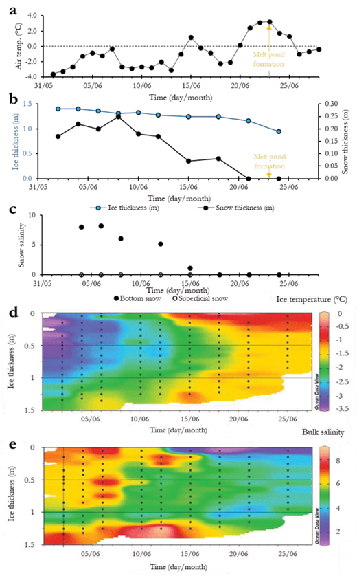
Temporal changes in environmental conditions in the sampling area. (a) Daily averaged air temperature obtained from the meteorological station in Qikiqtarjuaq between June 2 and June 28, (b) measured ice and snow thickness (snow disappeared from the sampling area after June 21), (c) bottom snow salinity (0.05-m layer directly in contact with sea ice) (closed circles) and superficial snow salinity (0.05 m layer at the top of the snow cover) (open circles) measured between June 4 and 23, (d) contour plot of sea-ice temperature, and (e) contour plot of sea-ice salinity. Black marks in the contours plots indicate actual sampling depths within the ice profiles. DOI: https://doi.org/10.1525/elementa.370.f2
Temporal changes in environmental conditions in the sampling area. (a) Daily averaged air temperature obtained from the meteorological station in Qikiqtarjuaq between June 2 and June 28, (b) measured ice and snow thickness (snow disappeared from the sampling area after June 21), (c) bottom snow salinity (0.05-m layer directly in contact with sea ice) (closed circles) and superficial snow salinity (0.05 m layer at the top of the snow cover) (open circles) measured between June 4 and 23, (d) contour plot of sea-ice temperature, and (e) contour plot of sea-ice salinity. Black marks in the contours plots indicate actual sampling depths within the ice profiles. DOI: https://doi.org/10.1525/elementa.370.f2
Average ice temperature calculated over the complete vertical profile increased from –3.30°C to –0.70°C at a rate of 0.08°C d–1 during the sampling period (Figure 2d). After June 15, sea ice became nearly vertically isothermal (at about –1.5°C), with the exception of the upper 0.2 m, which exhibited warmer temperatures of –0.5°C indicating important surface warming (0.15°C d–1) (Figure 2d).
Bulk-ice salinity decreased from about 9 to 1 during the sampling period (Figure 2e). The salinity decreased rapidly during the first sampling period (before June 15). From June 15 onward, fresher ice with salinity ≤2 was observed in the upper 0.1 m of the ice column. Locally, a visibly coarser and fresher superimposed ice layer of 0.06-m thickness (0.03–0.10-m) was observed after June 15. Superimposed ice forms when percolating snow meltwater re-freezes at the snow-ice interface (e.g., Kawamura et al., 2001).
The brine volume fraction (Vbr) ranged between 6% and 33% during the sampling period (Figure 3a), indicating that sea ice was permeable throughout the study (Golden et al., 1998). Before June 15, Vbr was ~10% in interior sea ice, and generally exceeded 15% throughout the ice column thereafter. Highest values of Vbr (~20%) were observed in the bottommost layers of the sea ice (0.1–0.2 m) and resulted from the direct influence of relatively warmer seawater. The minimum Vbr observed at the ice surface on June 18 corresponded to the presence of a superficial layer of coarser superimposed ice following the onset of snow melt. Additionally, melt-pond formation induced the percolation and subsequent refreezing of freshwater (Polashenski et al., 2017) which locally drastically reduced the Vbr after June 23.

Temporal variations in sea-ice physical characteristics. Contour plots of (a) brine volume fraction (%) calculated using Leppäranta and Manninen (1988) and Petrich and Eicken (2010), (b) brine salinity calculated using the formulation of Notz (2005), and (c) Rayleigh number using Notz and Worster (2008). Black marks indicate the depth corresponding to the calculated value within the ice profiles. DOI: https://doi.org/10.1525/elementa.370.f3
Temporal variations in sea-ice physical characteristics. Contour plots of (a) brine volume fraction (%) calculated using Leppäranta and Manninen (1988) and Petrich and Eicken (2010), (b) brine salinity calculated using the formulation of Notz (2005), and (c) Rayleigh number using Notz and Worster (2008). Black marks indicate the depth corresponding to the calculated value within the ice profiles. DOI: https://doi.org/10.1525/elementa.370.f3
Brine salinity profiles are indicative of the vertical (in)stability within the brine network (Notz and Worster, 2009). Before June 15, a strong vertical gradient was observed in the brine salinity profiles (Figure 3b) as saline brines (>40) stood above relatively less saline brines (<30). After June 15, brine salinity decreased to values between 3 and 35, with the lowest values measured in the uppermost ice layer, resulting in a stable (stratified) brine profile.
Ra values ranged from 5 to 18 before June 15 with the highest value observed in the ice surface layers (Figure 3c). After June 15, Ra values dropped drastically and stayed close to 0 for the rest of the sampling period (Figure 3c). This pattern is in agreement with the brine instability observed during the first half of the sampling period (prior to June 15) which, combined with the permeable state of the sea ice, indicates that the brine network was prone to desalination through the full ice depth via gravity drainage (Tison et al., 2010). Lower Ra numbers coincided with the stratification of the brine network from June 15, indicating the end of gravity drainage processes.
In summary, sea ice became progressively nearly isothermal and isohaline during the sampling period. The brine system dynamics transited from a vertically unstable gravity drainage phase before June 15 to a vertically stable phase after June 15 due to seasonal ice warming.
Temporal variations of Chl a and DMS concentrations in bottom sea ice and under-ice water
Chl a concentration in the bottom 0.1 m of sea ice was at maximum (380 µg L–1) on June 4 and decreased to reach its minimum value of 21 µg L–1 on June 21 (Figure 4a), which corresponds to a loss of 94% of ice Chl a concentration. Thereafter, concentrations of bottom-ice Chl a remained relatively low (21–31 µg L–1). Pelagic Chl a concentration at 0.5 m below the ice increased from 0.08 to 1.00 µg L–1 between June 2 and June 15, and then decreased to 0.62 µg L–1 on June 24 and June 27 (Figure 4b). Corresponding Chl a concentrations measured directly at the ice-water interface on June 24 and 27 reached 1.05 µg L–1 and 1.88 µg L–1, respectively.
The concentrations of DMS peaked at 814 ± 37 nmol L–1 in the bottom 0.1 m of sea ice at the beginning of the sampling and decreased abruptly by June 5, stabilizing at 255 ± 48 nmol L–1 (n = 7) for the rest of the sampling period (Figure 4c). Overall, no significant correlation was found between bottom-ice DMS and Chl a concentration (rs = 0.57; p = 0.12; n = 8). DMS concentrations in under-ice water varied between 1.6 and 5.6 nmol L–1 during the sampling period (Figure 4d). Concentrations of DMS directly at the ponded ice-seawater interface reached 3.8 nmol L–1 and 6.6 nmol L–1 on June 24 and 27, respectively.
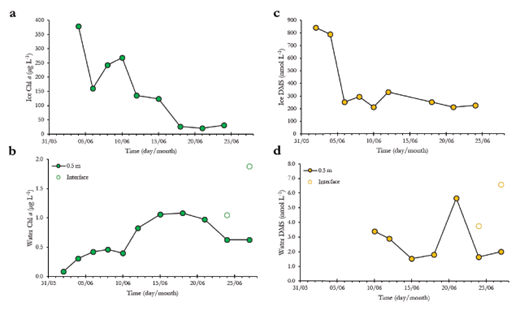
Temporal variations in Chl a and DMS concentrations in sea ice and under-ice water. (a) Chl a concentrations (µg L–1) in the bottom 0.1 m of sea ice, (b) Chl a concentrations (µg L–1) in under-ice water at 0.5 m (closed circles) and directly at the ice-water interface under melt ponds (open circles), (c) DMS concentrations (nmol L–1) in the bottom 0.1 m of sea ice, and (d) DMS concentrations (nmol L–1) in under-ice water at 0.5 m (closed circles) and directly at the ice-water interface under melt ponds (open circles). DOI: https://doi.org/10.1525/elementa.370.f4
Temporal variations in Chl a and DMS concentrations in sea ice and under-ice water. (a) Chl a concentrations (µg L–1) in the bottom 0.1 m of sea ice, (b) Chl a concentrations (µg L–1) in under-ice water at 0.5 m (closed circles) and directly at the ice-water interface under melt ponds (open circles), (c) DMS concentrations (nmol L–1) in the bottom 0.1 m of sea ice, and (d) DMS concentrations (nmol L–1) in under-ice water at 0.5 m (closed circles) and directly at the ice-water interface under melt ponds (open circles). DOI: https://doi.org/10.1525/elementa.370.f4
Temporal variations of DMS concentrations in snow, upper sea ice and interior sea ice
The levels of DMS were below the quantification limit (0.2 nmol L–1) in surface snow but varied between 0.3 and 15.5 nmol L–1 in the slush-snow layer directly in contact with the underlying sea ice (Figure 5a). DMS concentrations in the upper 0.1 m of the sea ice were constantly low (<30 nmol L–1) before June 15 (i.e., brine gravity drainage phase). After June 15 and during the whole brine stratification period, we observed high variability of surface-ice DMS concentrations, which notably peaked at 87 and 103 nmol L–1 on June 18 and 24, respectively (Figure 5b). In the interior sea ice (i.e., excluding bottom 0.1-m sea ice), DMS concentrations were relatively low (<0.3 and 30 nmol L–1) from the start of the sampling up to June 15 (i.e., end of the brine gravity drainage phase), and then increased to reach values as high as 109 nmol L–1 (i.e., during the stable phase) (Figure 5c).
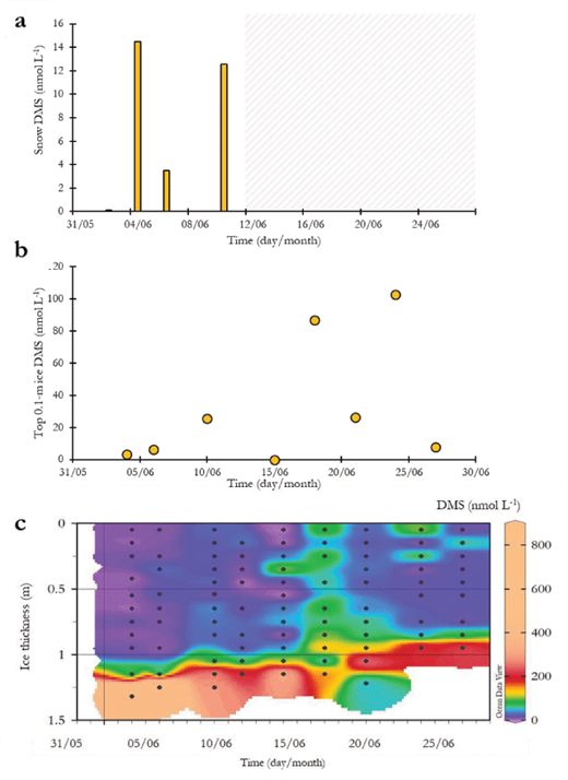
DMS concentrations in the snow and sea ice. (a) DMS concentrations (nmol L–1) in bottom snow between June 2 and 12 (no DMS measurements in were taken during the period marked with a shaded area), (b) DMS concentrations (nmol L–1) in the top 0.1-m of the ice, and (c) contour plot of bulk-ice DMS concentrations (nmol L–1). DOI: https://doi.org/10.1525/elementa.370.f5
DMS concentrations in the snow and sea ice. (a) DMS concentrations (nmol L–1) in bottom snow between June 2 and 12 (no DMS measurements in were taken during the period marked with a shaded area), (b) DMS concentrations (nmol L–1) in the top 0.1-m of the ice, and (c) contour plot of bulk-ice DMS concentrations (nmol L–1). DOI: https://doi.org/10.1525/elementa.370.f5
Physicochemical and biological characteristics of melt ponds
The three melt ponds sampled on June 24 were shallow (0.10–0.15 m), with lengths and widths that varied between 3 and 12 m and between 1.5 and 7 m, respectively (Table 1). Temperature in the melt ponds varied between –0.18 and 0.92°C, while salinity ranged from 0.3 to 2.0. Chl a concentrations ranged from 0.27 to 1.46 µg L–1, and DMS concentrations from 0.2 to 3.6 nmol L–1. Salinity, Chl a and DMS followed parallel trends in the sampled melt ponds (Table 1).
Physical and biological characteristics of the melt ponds sampled on June 24, 2015. DOI: https://doi.org/10.1525/elementa.370.t1
| Latitude (°N) | Longitude (°E) | Melt pond number | Length (m) | Width (m) | Depth (m) | Temp. (°C) | Salinity | Chl a(µg L–1) | DMS (nmol L–1) |
|---|---|---|---|---|---|---|---|---|---|
| 67.47583 | –63.78923 | MP1 | 12 | 1.5 | 0.10 | –0.18 | 0.3 | 0.27 | 0.2 |
| 67.47583 | –63.78788 | MP2 | 4 | 7.0 | 0.10 | –0.92 | 0.6 | 0.41 | 0.7 |
| 67.47550 | –63.78715 | MP3 | 3 | 2.5 | 0.15 | –0.23 | 2.0 | 1.46 | 3.6 |
Discussion
We investigated the temporal variations in DMS concentrations during the late melting period within various sea-ice related habitats, including snow, sea ice, under-ice water and melt ponds. Our results highlight the presence of DMS in all investigated environments, and the interconnectivity between the under-ice water, the bottom of sea ice, the interior of the ice, the snow and the atmosphere.
Our sampling captured the temporal succession between two distinct phases in sea-ice dynamics: (1) a brine gravity drainage phase from the start of the sampling up to June 15, followed by (2) a brine vertical stabilization phase when flushing occurred that extended from June 15 until the end of the sampling period. Gravity drainage is a process whereby sea ice undergoes desalination as cold and hypersaline (i.e., dense) brines are driven from the ice and replaced by seawater through convective movements. Flushing is described as the percolation of meltwater through the warming sea ice (Jardon et al., 2013). These two regimes of brine dynamics influenced (1) the exchange of biomass between sea ice and the underlying water column and (2) the exchange of DMS at the ice-water and ice-atmosphere interfaces. In the following sections, we discuss the exchange of biomass and DMS at the ice-seawater interface, and we review DMS dynamics in internal sea-ice layers and the existence of potential sea ice-atmosphere fluxes. We then show how snow and melt ponds could be transient sources of DMS for the atmosphere, and finally compare the estimated ice-to-atmosphere fluxes of DMS to potential sea-to-air fluxes.
Biochemical exchanges between sea ice and the under-ice water during the gravity drainage phase
The connectivity between the bottom of the ice and under-ice water is difficult to assess in the absence of thorough measurements of water circulation patterns under the ice and a proper evaluation of the spatial heterogeneity of the bottom ice itself at a relevant spatial scale (several kilometers). For this reason, we limit our interpretations to the salient features.
The Chl a concentrations measured at the bottom of the ice during our study, which ranged between 21 and 350 µg L–1 (i.e., 1.8 to 40.1 mg m–2; Figure 4a), fall in the lower range of reported values for bottom FYI at higher latitudes in the Arctic (3–450 mg m–2; Gosselin et al., 1997; Nozais et al., 2001; Fortier et al., 2002; Galindo et al., 2014). Such low Chl a concentrations suggest that the sampling took place during the decline of the ice-algal bloom associated with the snow-melt period (Galindo et al., 2017). Accordingly, Chl a concentrations at the bottom of the ice decreased by ~70% throughout the gravity drainage phase. This loss of ice algae from the bottom sea ice coincided with an increase in Chl a concentration in the under-ice water from 0.08 to 1.01 µg L–1 (Figure 4b). Removal of algal biomass from the bottom ice by gravity drainage and ice ablation (~30% loss in sea-ice thickness throughout the study) is consistent with the strong negative correlation observed between Chl a concentrations in bottom ice and under-ice water during the gravity drainage phase (rs = –0.88; p < 0.05; n = 7). Similar increases in under-ice water Chl a, as a result of sloughing of ice algae from the bottom ice, have been reported previously in the Arctic (e.g., Galindo et al. 2014; Mundy et al., 2014).
The potential contribution of ice algae to the build-up of biomass in the under-ice water during the gravity drainage phase was further explored by calculating the expected increases in Chl a concentration in the under-ice water due to ice-algal release. To do so, bulk-ice Chl a concentrations (µg L–1) were first converted to brine Chl a concentrations (µg L–1) following Tison et al. (2010). Briefly, bulk-ice Chl a concentrations were multiplied by the theoretical density of pure ice (0.91; Timco and Frederking, 1996) and divided by the average Vbr observed during gravity drainage phase (~20%). Assuming no water mass advection and a mixed layer depth of 20 m at our sampling site (Oziel et al., 2019), the release of Chl a from bottom ice could have resulted in an approximate 1.1 µg L–1 increase in under-ice water Chl a between June 4 and June 12. This value is almost twice the Chl a increase (0.6 µg L–1) measured in under-ice water during the corresponding period. The release of algal biomass from the bottom ice could thus entirely explain the net increase in Chl a in the upper mixed layer during the gravity drainage period. The Chl a released from the bottom ice and not recovered in under-ice water may have been advected horizontally, diluted by the increasing ice meltwater input, exported below the mixed layer or consumed by diverse heterotrophic micro- to macro-organisms. The above calculations assume no phytoplankton growth underneath the ice at this period due to the presence of a thick snow cover limiting light availability in the water column (Galindo et al., 2017).
Maximum DMS concentrations in the ice were measured in the bottom ice layer, with values varying between 212 and 840 nmol L–1 (Figures 4c and 5c). This distribution of DMS within sea ice is expected considering its biogenic origin. The DMS peaks in bottom ice compare well with the maximum value of 769 nmol L–1 measured in FYI of the Amundsen Gulf during spring (Carnat, 2014) and are also in the same range as maximum DMS concentrations reported in Antarctic bottom ice (370–1400 nmol L–1; Tison et al., 2010; Carnat et al., 2014). As observed for Chl a, DMS concentrations were highest at the beginning of the sampling period and decreased by 60% during the gravity drainage phase.
High levels of bottom-ice DMS such as observed during our study could represent a potential source of DMS for under-ice water. DMS concentrations in the under-ice water at 0.5 m ranged between 1.53 and 5.65 nmol L–1. Under-ice water DMS concentrations were also measured directly at the ice-water interface on June 24 and 27 (Figure 4d). On these two dates, interface DMS concentrations were two to three times higher than the corresponding values measured at 0.5 m. Such a gradient of DMS concentration between bottom ice, interface seawater and under-ice seawater at 0.5 m suggests that gravity drainage and ice ablation favored the transfer of DMS from the ice to the water column. Unfortunately, the absence of DMS measurements for under-ice water before June 10 and the low sampling frequency (2–3 days) associated with the notoriously rapid turnover rate of DMS (h–1; e.g., Wolfe et al., 1999) do not permit a thorough estimation of the contribution of bottom-ice DMS to the DMS pool measured in the underlying water column. However, the hypothesis of DMS transfer from bottom ice to under-ice water is consistent with Antarctic studies, which report that the gravity drainage during the melt season was associated with significant loss of DMS from sea ice resulting in DMS peaks in the under-ice water column (DiTullio et al., 2000; Trevena and Jones, 2006; Tison et al., 2007, 2010). Accordingly, DMS concentrations as high as 24 nmol L–1 have been measured in under-ice water during the spring-summer transition in the Antarctic (Carnat et al., 2014). While part of the DMS was lost to the underlying seawater, the persistence of high DMS concentrations (>200 nmol L–1) in bottom ice throughout the study, despite the sharp reduction of ice-algal biomass, might appear somewhat surprising. Such a discrepancy suggests that mechanisms involved in biomass (particle) removal from the ice (i.e., gravity drainage, ice ablation and flushing) did not affect bottom-ice DMS concentrations (dissolved and gaseous states) to the same extent. Chl a-containing particles may have sunk in the water column while DMS remained in solution or in the gas phase. The potential DMS transport in the gaseous state is further explored later in the discussion.
DMS dynamics in interior sea ice
DMS concentrations in the interior ice remained below 30 nmol L–1 during the brine gravity drainage phase compared to bottom-ice concentrations. Interior-ice DMS concentrations increased sharply on June 15, when the ice column became nearly isohaline and isothermal during the vertically stable brine phase (Figure 5c).
The in situ production of DMS by an active microbial community in interior sea ice was likely not the main driver of the increase in DMS during the vertically stable phase (from June 15). Even though interior-ice Chl a concentrations could not be obtained during this study due to logistical constraints, this interpretation is backed by the following arguments. First, DMS concentrations were minimal in interior sea ice before June 15, suggesting the absence of large pre-established DMS-productive assemblages within sea ice. Second, the loss of brine during the first half of the sampling period until June 15 is likely to have displaced most of the algae in sea ice toward under-ice water (Lavoie et al., 2005; Mundy et al., 2005). Third, in the Arctic, more than 95% of ice-algal communities and DMSP pools are concentrated within the bottom-ice layer (Levasseur et al., 1994; Galindo et al., 2014). In Antarctic sea ice, microbial communities thriving in the upper ice layers, far from direct contact with seawater, are supported by flooding events that lead to heightened levels of salinity (and DMS) within the interior sea ice (Asher et al., 2011; Carnat et al., 2014; Damm et al., 2016). Such flooding events are seldom reported in the Arctic (Petrich and Eicken, 2010) and were not observed during our study (constantly positive freeboard). For these reasons, we argue that DMS production in the interior ice during the vertically stable phase was most probably minimal and did not contribute substantially to the observed increase in DMS. Instead, our results suggest that the increase in interior sea-ice DMS after June 15 resulted from the upward transport of this gas from the DMS-rich bottom sea ice.
During our study, brine density instability combined with sea-ice permeability (Figure 3) led to the desalination of the entire ice column through gravity drainage (Notz and Worster, 2009). Most of the gravity drainage activity occurred before June 15 as indicated by the strong vertical gradient in Ra numbers profiles, with relatively higher Ra values in the upper sea ice (Figure 3c). After June 15, surface warming led to the development of isothermal profiles in sea ice, resulting in the stratification of the brine network. During this vertically stable phase, sea-ice permeability continued to increase except where surface meltwater infiltration formed a coarser superimposed ice layer (June 18) (Figure 3a).
Given the absence of large sources of DMS in the upper sea-ice layer, our results suggest that the increase in DMS concentrations in internal and surface-ice layers was predominantly driven by the changes in sea-ice microstructure allowing upward transport of DMS from the bottom of the ice. The transition from gravity drainage to vertical stabilization within the ice microstructure influenced the distribution of DMS concentrations in sea ice. The concentrations of DMS in the interior ice (i.e., excluding the high DMS values measured in the bottommost 0.1–0.2-m layers) significantly increased with ice temperature (rs = 0.44; p < 0.05; n = 74) (Figure S1) and decreased with increasing brine salinity (Figure S2) (rs = –0.44; p < 0.05; n = 74) and Ra number (rs = –0.49; p < 0.05; n = 65) (Figure S3). These correlations are consistent with our interpretation that sea-ice warming favored the upward movement of DMS from bottom ice to the atmosphere as the pool of bottom-ice DMS remained important throughout the melt season (<200 mmol L–1). They are also consistent with Tison et al. (2010), who suggested the occurrence of DMS diffusion through Antarctic ice and across the ice-atmosphere interface under a stratified and permeable brine regime similar to the conditions encountered during our vertically stable phase.
No significant relationship was found between Vbr and DMS (rs = –0.23; p = 0.053; n = 74) (Figure S4), which suggests that, once Vbr surpasses a permeability threshold (8% from sampling day 1 onwards; Figure 3a), the establishment of a stable stratified brine network allows for DMS diffusion within sea ice, rather than further increases in ice permeability (i.e., Vbr). However, the presence of impermeable ice layers can restrain DMS transport within sea ice. This effect is illustrated by the observed accumulations of 87 and 109 nmol DMS L–1 in the upper 0.1 m of sea ice on June 18 and June 24, respectively (Figure 5b). On June 18, surface sea-ice permeability had decreased strongly due to the formation of a superimposed ice layer caused by the infiltration and subsequent refreezing of surface meltwater on sea ice. On June 24, the DMS ice core was sampled directly inside a melt pond, where freshwater ice layers are known to form at the ice-melt pond interface allowing the persistence of melt ponds on positive-freeboard ice which is otherwise highly permeable (Polansky et al., 2017). Our interpretation of these accumulations of DMS under impermeable layers on June 18 and 24 is consistent with Nomura et al. (2012), who reported a significant decrease in DMS outgassing from sea ice above locally impermeable layers in the Antarctic. The formation of transiently impermeable ice layers during the vertically stable phase may thus impede DMS outgassing across the ice-atmosphere interface and cause a temporary DMS build-up in the upper part of the ice column.
DMS transport through sea ice
As our results suggest that the increase in interior sea-ice DMS after June 15 resulted from the upward transport of this gas from the DMS-rich bottom sea ice, the following sections present an estimation of: (1) DMS transport coefficients D (DDMS/br for molecular diffusion in brine and DDMS/ice for transport in bulk ice); and (2) DMS fluxes across the sea ice-atmosphere interface.
First, since no parameterization exists for the transport of DMS in sea ice and no diffusion coefficient for DMS in sea ice has been reported in the literature, we computed an in situ diffusion coefficient (DDMS) based on the temporal variation of DMS concentrations in sea ice and Fick’s Law of diffusion. We used and compared two different approaches. For the first approach we computed an in situ molecular diffusion coefficient in brine (DDMS/br) assuming that all of the DMS measured in melted sea-ice samples was initially concentrated in the brine and transported in the dissolved state in the brine. For the second approach, we computed a bulk-ice transport coefficient (DDMS/ice) from the bulk-ice DMS concentration measured in melted sea-ice samples. In the second approach, the gaseous phase transport is also potentially involved. Second, we present and compare the computation of potential DMS flux (F) using (1) DDMS/br and (2) DDMS/ice, as well as D values reported in the literature (Table 2).
Comparison of molecular diffusion and bulk-ice transport coefficients from the literature and this study. DOI: https://doi.org/10.1525/elementa.370.t2
| Gas | Literature | D value (10–5 cm2 s–1) | Environment | Type of coefficient | Coefficient conditions |
|---|---|---|---|---|---|
| DMS | Saltzman et al., 1993 | 0.69 | Seawater at 0°C | Molecular diffusion | D = Ae–Ea/RT |
| DMS | Shaw et al., 2011 | 0.65 | Seawater at –1.85°C | Molecular diffusion | \[D = 7.4{10^{ - 8}}{\textstyle{{{{(\phi \, \times \,{M_{DMS}})}^{0.5}}T} \over {{n_{w}}V_B^{0.6}}}}\] |
| DMS | This study | 5.2 ± 51a | Natural melting sea ice | Molecular diffusion | –0 < T (°C) < –2.5, 6% < Vb < 33% |
| SF6 | Loose et al., 2011 | 13 ± 40b | Artificial growing sea ice | Bulk transport, in situ observation | –4 < T (°C) < –12, 6% < Vb < 8% |
| O2 | Loose et al., 2011 | 3.9 ± 41b | Artificial growing sea ice | ||
| N2 | Crabeck et al., 2014 | 2.49 ± 11a | Natural steady-state sea ice | Bulk transport, in situ observation | –3.5 > T (°C) < –2, 5.4% < Vb < 8.05% |
| O2 | Crabeck et al., 2014 | 1.5 ± 9a | Natural steady-state sea ice | ||
| DMS | This study | 33 ± 41a | Natural melting sea ice | Bulk transport, in situ observation | 0 < T (°C) < –2.5, 6% < Vb < 33% |
Estimation of in situ DMS transport coefficients
DMS molecular diffusion coefficient in brine, DDMS/br
Based on Fick’s Law of diffusion and temporal changes in DMS concentrations in the sea-ice cover, it is possible to deduce an in situ molecular diffusion coefficient (DDMS/br) between successive ice layers sampled within a vertical ice profile using the brine DMS concentration gradient (ΔC = Δ[DMS]br):
where F (µmol m–2 d–1) is the DMS flux in or out of each 0.1-m ice section between June 15 and June 18 (Figures 6a and b). The flux F was computed as the difference between DMS burdens in µmol m–2 of ice cover between the cores sampled on June 15 and June 18 (Figure 6a) divided by the time in days (d) for each of the 0.1-m ice layers of the vertical ice profile sampled (Figure 6b). DMS burdens in µmol m–2 of ice cover were inferred from brine DMS concentration (µmol L–1 of brine) that were multiplied by the exact volume of brine contained in each 0.1-m ice section and divided by the surface of an ice core in m2 (r = 0.045 m). Note that DMS burdens in µmol m–2 of ice cover can also be inferred from bulk-ice DMS concentration (µmol L–1 of ice). In this case [DMS]ice (µmol L–1 of ice) is multiplied by the exact volume of ice sampled and divided by the surface of an ice core in m2 (r = 0.045 m); Zice is the thickness of the ice layers sampled (0.1 m); and ΔC is the difference in DMS brine concentrations observed between June 15 and June 18 in brines ([DMS]br J18–[DMS]br J15) for each 0.1-m ice layer. Values for DDMS/br obtained from Equation 5 are shown in Figure 6c.
![Figure 6. Calculation of the DMS flux and diffusion coefficient in brine. (a) Profiles of DMS concentration (μmol m–2) in the sea-ice cover on June 15 and June 18, showing DMS accumulation in the internal ice layer (0 to 1 m) and loss of DMS from the bottom ice (1.0 to 1.25 m) due to upward diffusion across the ice cover, with total amount gained in the internal layer and lost from the bottom layer shown in the insert; (b) DMS fluxes in or out of each 0.1-m ice layer computed as the difference of DMS quantities between June 15 and June 18 as shown in panel (a) divided by the time in days; (c) computed diffusion coefficient DDMS/br for each 0.1-m ice layer, using Equation 5, the DMS flux F in panel (b), and the difference in DMS quantities observed between June 15 and June 18 ([DMS]br J18–[DMS]br J15) for each 0.1-m ice layer. DOI: https://doi.org/10.1525/elementa.370.f6](https://ucp.silverchair-cdn.com/ucp/content_public/journal/elementa/7/10.1525_elementa.370/6/m_370-6390-1-pb.png?Expires=1716293310&Signature=ET~JfbKms~-m232j7YbqJ6FEUSC5HHeD6tyj2a1fJjmh9XFEjzzGsUByCWAbZrQwt-1D6Oc~7RG462QmzJ933Nd2iAm~~zTt9~RFLSt72OEGXiuWCN5qO-0XSd7Wh9N1n3c7ZRw1NOaNp63PrlicILaOb2dD89-Qpnup6bu-2KI7rIz1sMdVIgpsjerkOESLEyuKrpNCXfhSRi2lHE4cV2h7ZFSnFZJ4DF2WvWYC8YmG-oIMYeM6o5HAyW79K4QD6ZBOjU-Jbx4bc1aNxL~-gRhg5YJT~7cqARnh-1pIzAtnXwANxJMaqCjQC6OfApCUhjuGN2Afq1a4NK6rmCce9w__&Key-Pair-Id=APKAIE5G5CRDK6RD3PGA)
Calculation of the DMS flux and diffusion coefficient in brine. (a) Profiles of DMS concentration (μmol m–2) in the sea-ice cover on June 15 and June 18, showing DMS accumulation in the internal ice layer (0 to 1 m) and loss of DMS from the bottom ice (1.0 to 1.25 m) due to upward diffusion across the ice cover, with total amount gained in the internal layer and lost from the bottom layer shown in the insert; (b) DMS fluxes in or out of each 0.1-m ice layer computed as the difference of DMS quantities between June 15 and June 18 as shown in panel (a) divided by the time in days; (c) computed diffusion coefficient DDMS/br for each 0.1-m ice layer, using Equation 5, the DMS flux F in panel (b), and the difference in DMS quantities observed between June 15 and June 18 ([DMS]br J18–[DMS]br J15) for each 0.1-m ice layer. DOI: https://doi.org/10.1525/elementa.370.f6
Calculation of the DMS flux and diffusion coefficient in brine. (a) Profiles of DMS concentration (μmol m–2) in the sea-ice cover on June 15 and June 18, showing DMS accumulation in the internal ice layer (0 to 1 m) and loss of DMS from the bottom ice (1.0 to 1.25 m) due to upward diffusion across the ice cover, with total amount gained in the internal layer and lost from the bottom layer shown in the insert; (b) DMS fluxes in or out of each 0.1-m ice layer computed as the difference of DMS quantities between June 15 and June 18 as shown in panel (a) divided by the time in days; (c) computed diffusion coefficient DDMS/br for each 0.1-m ice layer, using Equation 5, the DMS flux F in panel (b), and the difference in DMS quantities observed between June 15 and June 18 ([DMS]br J18–[DMS]br J15) for each 0.1-m ice layer. DOI: https://doi.org/10.1525/elementa.370.f6
Calculation of DDMS/br was based on the temporal variations of DMS burden in µmol m–2 in the ice sampled between June 15 and June 18 (Figure 6a and b) for the following reasons: June 15 was the first day when diffusion could occur in sea ice, as the gravity drainage phase had ended (Figure 3c); and outgassing of the DMS potentially transported upwards was limited by the formation of an impermeable layer of superimposed ice at the surface of the ice on June 18 (Figures 3a and 6a). This impermeable layer resulted in the observed spike of DMS throughout the ice column (Figures 5c and 6a). Between June 15 and June 18, the upper part of the ice column (i.e., from the ice surface to down to 1 m) gained 31.6 µmol of DMS m–2, while the bottom of the ice (1.00–1.25 m) lost 19.6 µmol of DMS m–2 (Figure 6a).
Molecular diffusion of DMS in brine (DDMS/br) assumes that all of the DMS measured in the melted sea-ice sample was entirely in the dissolved state in the brine medium ([DMS]br = [DMS]ice × Vbr) and that all of the DMS was transported in its dissolved state through the brine network. As Vbr was relatively constant between June 15 and June 18, and the relative enrichments in DMS in brine and bulk ice were similar (Figure 7), no concentration or dilution effects were linked to the change of Vbr during our study. Therefore, the brine concentration gradient can be used to infer the diffusion coefficient using Fick’s Law (Equation 5).
![Figure 7. Relationship between the relative change in DMS concentration in bulk ice and in brine. Relative change of DMS in bulk ice and brine between June 15 and June 18 for each sampled depth computed as [DMS]br J18/[DMS]br J15 × 100 and [DMS]ice J18/[DMS]ice J15 × 100. Deviations from the 1:1 relationship indicate a change in brine concentration ([DMS]br) by dilution or concentration effect linked to change of brine volume. DOI: https://doi.org/10.1525/elementa.370.f7](https://ucp.silverchair-cdn.com/ucp/content_public/journal/elementa/7/10.1525_elementa.370/6/m_370-6391-1-pb.png?Expires=1716293310&Signature=x21ap7o2xp04MkNxJ-Vu6nnBJvxNjqCD3lL9IhSH40AghrUlE3O39KxVn8up5B9R1avTQOtwOt3lXjmoM2YmbyhV5LvsGV2cXdp5KIKcXK6Bd71XKJd6GejInPISWhdqPY~1Mj9tCubqNyiwQmhKO7z0AuBqaqz2yM-GbhLKLaewaaNcEvf3D0xQjtehicSDIByryN0~58pB~POT07JEQW4Z-8KWLJPi9fENKRNjqalaCiCfcCo8M1fUsugviB7y0dCz8uHAkoakt3nat8oxn1GqfQF1lnCJNpknDjojIj~ZPzWTdzCsG-aaPKbb9YH~Uw8gaLtkjpzok9VIkcluYw__&Key-Pair-Id=APKAIE5G5CRDK6RD3PGA)
Relationship between the relative change in DMS concentration in bulk ice and in brine. Relative change of DMS in bulk ice and brine between June 15 and June 18 for each sampled depth computed as [DMS]br J18/[DMS]br J15 × 100 and [DMS]ice J18/[DMS]ice J15 × 100. Deviations from the 1:1 relationship indicate a change in brine concentration ([DMS]br) by dilution or concentration effect linked to change of brine volume. DOI: https://doi.org/10.1525/elementa.370.f7
Relationship between the relative change in DMS concentration in bulk ice and in brine. Relative change of DMS in bulk ice and brine between June 15 and June 18 for each sampled depth computed as [DMS]br J18/[DMS]br J15 × 100 and [DMS]ice J18/[DMS]ice J15 × 100. Deviations from the 1:1 relationship indicate a change in brine concentration ([DMS]br) by dilution or concentration effect linked to change of brine volume. DOI: https://doi.org/10.1525/elementa.370.f7
DMS transport coefficient in bulk ice, DDMS/ice
Recent studies on sea ice (Loose et al., 2011; Crabeck et al., 2014; Moreau et al., 2014) have reported that gas transport is not limited to molecular diffusion in the dissolved state in brine solution. Gas transport may also take place in the gaseous state, i.e., as bubbles moving upwards under buoyancy within the brine network (Loose et al., 2011; Crabeck et al., 2014). From bulk-ice concentration gradients, Loose et al. (2011) computed an apparent transport coefficient for SF6 and O2 in growing artificial sea ice, and Crabeck et al. (2014) deduced DO2, DN2 and DAr in natural sea ice (Table 2). These previous studies reported in situ transport processes in sea ice and considered both liquid diffusion and gaseous phase transport as potential pathways for gas through sea ice. To take into account the potential transport of DMS by air bubbles, we inferred a transport coefficient for DMS in sea ice (DDMS/ice) between June 15 and 18 from the bulk-ice concentration gradient (ΔC = Δ[DMS]ice) instead of brine concentration gradient using Equation 5. The use of this approach no longer assumes that all of the DMS present is in the dissolved state in the brine.
In situ molecular diffusion of DMS in brine, computed using Equation 5 (Figure 6c) and the brine DMS concentration gradient Δ[DMS]br, yielded a mean molecular diffusion value (DDMS/br) of 5.2 × 10⁻⁵ cm2 s–1 ± 51% relative S.D. (n = 10). This computed in situ molecular diffusion in brine is an order of magnitude higher than molecular diffusion using seawater parameterization (Table 3 and Figure 8). Seawater parameterization proposed by Saltzman at 0°C, yielded a DDMS/br value of 0.69 × 10⁻⁵ cm2 s–1 (Table 3 and Figure 8), while the parameterization from Wilke and Chang (1955), used notably in Shaw et al. (2011) to compute fluxes of volatile organic iodine compounds in sea ice, yielded a DDMS/br of 0.65 × 10⁻⁵ cm2 s–1 (Table 3 and Figure 8). In situ bulk transport of DMS computed with Equation 5 and the bulk-ice DMS concentration gradient yielded a mean transport coefficient value (DDMS/ice) of 33 × 10–5 cm2 s–1 ± 41% relative S.D. (n = 10) (Table 3 and Figure 8). This value is in the same order of magnitude as DSF6 values reported by Loose et al. (2011) but is 10 times larger than DO2 and DN2 values reported by Crabeck et al. (2014) (Table 3 and Figure 8).
DMS upward transport from bottom ice and surface ice using brine and bulk DMS concentrations. DOI: https://doi.org/10.1525/elementa.370.t3
| Calculation of DMS molecular diffusion flux (Fbr) using Δ[DMS]br from this study | |||
|---|---|---|---|
| DDMS/br (10–5 cm2 s–1) | Reference | Fbr from bottom iceb (μmol m–2 d–1, ΔZ = 1.0 ± 0.12 m) | Fbr from surface iceb (μmol m–2 d–1, ΔZ = 0.05 m) |
| 0.69 | Saltzman et al., 1993 | –0.05 ± 0.01b | –1.27 ± 0.65b |
| 0.65 | Shaw et al., 2011 | –0.05 ± 0.01b | –10.41 ± 0.04b |
| 5.2 ± 51%a | This study | –0.47 ± 0.08b | –9.30 ± 4.70b |
| Calculation of bulk DMS transport flux (Fice) using Δ[DMS]ice from this study | |||
| DDMS/ice (10–5 cm2 s–1) | Reference | Fice from bottom iceb (μmol m–2 d–1, ΔZ = 1 ± 0.12 m) | Fice from surface iceb (μmol m–2 d–1, ΔZ = 0.05 m) |
| 13 ± 40%a | Loose et al., 2011 | –0.24 ± 0.06b | –2.13 ± 0.25b |
| 2.49 ± 11%a | Crabeck et al., 2014 | –0.05 ± 0.01b | –0.41 ± 0.05b |
| 33 ± 41%a | This study | –0.40 ± 0.15b | –5.50 ± 0.65b |
| In situ DMS fluxes reported over Antarctic sea ice | |||
| D value (10–5 cm2 s–1) | Reference | In situ DMS flux (μmol m–2 d–1) | Method |
| n/ac | Nomura et al., 2012 | 0.3–5.3 | Chambers |
| n/ac | Zemmelink et al., 2008 | 10–29 | Relaxed Eddy Accumulation |
a Mean ± relative standard deviation, n = 10.
b Mean ± relative standard deviation, n = 5.
c Not applicable.
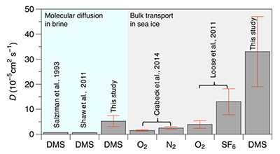
Comparative coefficients for gas molecular diffusion in brine and bulk transport in sea ice. Molecular diffusion coefficients in brine (green-shaded area) were computed using the parameterizations of Shaw et al. (2011), Salzman et al. (1993) and this study, with the latter involving in situ observations, Equation 5 and the brine concentration gradient. For this study, the mean and relative S.D. (error bar) of the in situ molecular diffusion coefficient (DDMS/br) are based on data presented in Figure 6c. Bulk transport coefficients (red-shaded area) were computed using the parameterizations of Crabeck et al. (2014), Loose et al. (2011) and this study. Mean and relative S.D. (errors bar) of the bulk transport coefficient (DDMS/ice) are reported from the work of Crabeck et al. (2014) and Loose et al. (2011). For this study, the relative S.D. of the in situ bulk-ice transport coefficient was computed in each ice layer based on profiles from June 15 and 18 using Equation 5 and the bulk-ice concentration gradient. DOI: https://doi.org/10.1525/elementa.370.f8
Comparative coefficients for gas molecular diffusion in brine and bulk transport in sea ice. Molecular diffusion coefficients in brine (green-shaded area) were computed using the parameterizations of Shaw et al. (2011), Salzman et al. (1993) and this study, with the latter involving in situ observations, Equation 5 and the brine concentration gradient. For this study, the mean and relative S.D. (error bar) of the in situ molecular diffusion coefficient (DDMS/br) are based on data presented in Figure 6c. Bulk transport coefficients (red-shaded area) were computed using the parameterizations of Crabeck et al. (2014), Loose et al. (2011) and this study. Mean and relative S.D. (errors bar) of the bulk transport coefficient (DDMS/ice) are reported from the work of Crabeck et al. (2014) and Loose et al. (2011). For this study, the relative S.D. of the in situ bulk-ice transport coefficient was computed in each ice layer based on profiles from June 15 and 18 using Equation 5 and the bulk-ice concentration gradient. DOI: https://doi.org/10.1525/elementa.370.f8
Strict molecular diffusion in water follows the Graham’s law relationship, which predicts faster diffusivity for gases with lower molecular weight. In water, DDMS has units of 10–6 cm2 s–1, while lighter species, such as O2, N2 and SF6, have molecular diffusion coefficients 10-fold faster with units of 10–5 cm2 s–1 (Stauffer et al., 1985). The in situ molecular diffusion coefficients (DDMS/br) computed here, assuming that the DMS is transported only in the dissolved state in brine, were approximately 5-fold higher than previously reported molecular diffusions coefficients for DMS in water.
Bulk-ice diffusion usually does not follow the Graham’s law relationship. Loose et al. (2011) found that the diffusion coefficient of SF6 (the heavier gas) was greater than that for O2 (lighter than SF6). According to Loose et al. (2011), gas solubility might have a greater influence than gas kinetics on diffusion in sea ice. Gases with the lowest solubility would preferentially accumulate in air bubbles, which can enhance the bulk transport depending on the amount of gas-filled pore space. Gas in the gaseous phase diffuses faster by three orders of magnitude compared to gas in the dissolved state in solution (i.e., molecular diffusion). In situ bulk transport coefficients (DDMS/ice) calculated for this study were of the same order of magnitude as DSF6/ice (Loose et al., 2011), and 10 times greater than DN2/ice (Crabeck et al., 2014) (Table 2). These results are somewhat unexpected, as DMS is much more soluble than SF6 and N2 (Dacey et al., 1984; Garcia and Gordon, 1992; Johnson 2010).
According to Dacey et al. (1984), atmospheric DMS is far from equilibrium with seawater and displays DMS partial pressure four times higher than predicted by the solubility equilibrium. The transport of DMS through bubble buoyancy should then be smaller than for SF6 and O2, leading to a smaller in situ bulk transport coefficient for DMS than what is observed. However, the following considerations can enlighten this apparent discrepancy. First, bulk gas transport in sea ice also depends on the geometry of the brine network (Loose et al., 2011; Zhou et al., 2013; Crabeck et al., 2014; Moreau et al., 2014). Larger and less tortuous channels would lead to higher bulk transport. Both studies from Crabeck et al. (2014) and Loose et al. (2011) took place before the onset of sea-ice melt and at lower Vbr than in this study (Table 2), which would explain why bulk transport of DMS might be potentially higher at our sampling site. Second, even if only a small fraction of DMS present in the brine system is expected to partition into the gaseous phase, bubbles may mediate upward DMS transport because the brine network may become increasingly filled with air during the melt period as a result of ice melt (Zhou et al., 2013; Crabeck et al., 2019). As Vbr increases during the melt period, gaseous inclusions are expected to increase (Crabeck et al., 2019) and connect to each other. While higher molecular weight and the solubility of DMS suggest that our computations of in situ DDMS/br and DDMS/ice might be overestimated, larger Vbr and potentially higher bubble content linked to sea-ice melt probably enhanced upward transport of DMS in our study. Bubble formation in the brine systems of FYI may therefore become highly relevant for DMS transport during the development and decline of ice-algal blooms, when DMS may be continuously supplied through metabolic reactions within the microbial community. The subsequent rising of buoyant bubbles is therefore expected to increase upward diffusion of DMS under warm ice conditions during the melt period.
Estimates of DMS flux towards the atmosphere
Fluxes from bottom ice
Potential diffusive fluxes (F) of bottom-ice DMS through the ice column were estimated using Fick’s first Law of diffusion as in Loose et al. (2011) under the assumption of steady state (Equation 6):
where F is the estimated diffusion flux of DMS expressed in µmol m–2 d–1, D is the diffusion coefficient; A is the surface area in m², zice is the full ice thickness (1.1 ± 0.12 m, n = 5), and Ca is the DMS concentration in the air above sea ice in mol m–3. Ca was set to zero, as it is negligible compared to the bottom-ice DMS concentrations. C is the bottom DMS concentration in (1) mol m–3 of brine ([DMS]br) or (2) mol m–3 of ice ([DMS]ice). For case (1), F was computed using the brine concentration gradient and DDMS/br (Fbr), while in case (2) we used the bulk-ice concentration gradient and DDMS/ice to calculate flux in ice (Fice).
After June 15, with the onset of the vertically stable phase and assuming that all DMS was diffusing in dissolved state in the brine, the average DMS flux Fbr estimated from bottom brine DMS concentrations and in situ molecular coefficient (DDMS/br) was 0.47 ± 0.08 µmol m–2 d–1 (n = 5), which is an order of magnitude higher than F calculated using D value from seawater parametrization from Saltzman et al., 1993. (Table 3). For the same period, the average Fice estimated from bottom bulk-ice DMS concentrations and in situ bulk transport coefficient (DDMS/ice) was 0.40 ± 0.15 µmol m–2 d–1 (n = 5), which compares well with the Fice of 0.24 ± 0.06 µmol m–2 d–1 (n = 5) computed with the bulk transport coefficient (DSF6/ice) from Loose et al. (2011) (Table 3). However, these F values are an order of magnitude higher than the mean of 0.05 ± 0.01 µmol m–2 d–1 (n = 5) computed for N2 using bulk transport coefficient (DN2/ice) from Crabeck et al. (2014). Such comparisons of F computed using DDMS from this study against various F calculated using D values obtain from the literature serve two purposes: they give information on the sensitivity of F to variations in the diffusion coefficient D, and they serve as markers to evaluate our results in the context of other published literature. Finally, our F values computed with the in situ molecular diffusion coefficient (DDMS/br) versus the in situ bulk transport coefficient (DDMS/ice) from the brine concentration gradient and bulk-ice concentration gradient, respectively, compared well (Table 3). These two approaches yielded similar F values (Table 3 and Figure 9) because the effects of lower diffusion values in the case of molecular diffusion in brine were offset by steeper concentration gradients between the bottom layer and the atmosphere (Table 3). Over time and independently of the computational approach (in situ molecular diffusion versus in situ bulk transport), F ranged from 0.3 to 0.8 µmol m–2 d–1 (Figure 9). Smaller F values were observed on June 18 when DMS concentrations of both bottom bulk ice and brine were low (155 nmol L–1 of ice and 876 nmol L–1 of brine) (Figure 9).
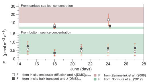
Estimated DMS flux for each sampling day between June 15 and 27. Mean DMS flux F and relative standard deviation (error bars) for each sampling day between June 15 and 27, using computed in situ molecular diffusion (white symbols, DDMS/br: 5.2 ± 51% 10–5 cm2 s–1, n = 10) and computed in situ bulk-ice transport coefficient (grey symbols, DDMS/ice: 33 ± 41% 10–5 cm2 s–1, n = 10). Circles indicate F computed from bottom-ice DMS brine concentrations; squares indicate F computed from surface-ice DMS. The red- and green-shaded areas show the range of F observed at the ice-atmosphere interface by Zemmelink et al. (2008) and Nomura et al. (2012) by eddy correlation and chamber measurements, respectively. DOI: https://doi.org/10.1525/elementa.370.f9
Estimated DMS flux for each sampling day between June 15 and 27. Mean DMS flux F and relative standard deviation (error bars) for each sampling day between June 15 and 27, using computed in situ molecular diffusion (white symbols, DDMS/br: 5.2 ± 51% 10–5 cm2 s–1, n = 10) and computed in situ bulk-ice transport coefficient (grey symbols, DDMS/ice: 33 ± 41% 10–5 cm2 s–1, n = 10). Circles indicate F computed from bottom-ice DMS brine concentrations; squares indicate F computed from surface-ice DMS. The red- and green-shaded areas show the range of F observed at the ice-atmosphere interface by Zemmelink et al. (2008) and Nomura et al. (2012) by eddy correlation and chamber measurements, respectively. DOI: https://doi.org/10.1525/elementa.370.f9
F values computed using in situ DDMS/br and DDMS/ice (Table 3 and Figure 9) are low in comparison with those measured over Antarctic sea ice by Nomura et al. (2012) using the flux chamber approach (0.3 to 5.3 µmol m–2 d–1) and by Zemmelink et al. (2008) using the Relaxed Eddy Accumulation approach (<10 to 29 µmol m–2 d–1) (Figure 9). The presence of DMS-rich slush layers on top of the Antarctic sea ice may explain the higher fluxes reported by these authors, as our calculation only takes into account the DMS present at the bottom of the ice. Our computed F values are also moderated by the thickness of the ice cover (i.e., thickness of the diffuse layer). The presence of impermeable layers at the top of the ice on June 18 and June 24 prevented the outgassing of DMS to the atmosphere, which enabled the observation of high DMS concentrations reaching >100 nmol L–1. We calculated that the removal of these temporary barriers to diffusion would result in instantaneous fluxes at least 10 times higher than DMS fluxes from bottom sea ice, with F values above 1 µmol m–2 d–1 independently of the D value used for the computation (Table 3 and Figure 9). Using in situ DDMS/br and DDMS/ice, we computed average fluxes of 9.3 ± 4.7 µmol m–2 d–1 (n = 5) and 5.5 ± 0.65 µmol m–2 d–1 (n = 5), respectively, which are more in line with the fluxes measured over Antarctic sea ice (Table 3 and Figure 9). While DMS concentrations of bottom and surface brine were similar for June 18 and June 24, F computed from the surface-ice layers was substantially higher than that calculated from the bottom-ice layers, because the thickness of the diffusive layer is smaller for the surface-ice layer (Table 3).
Fluxes from snow and melt ponds
The wicking of DMS-containing brine from surface sea ice into the snow cover might be an additional pathway for the release of DMS to the atmosphere. Discrete sampling of bottom slush-snow between June 2 and June 12 indicated highly variable DMS concentrations in this environment (0.3–15.5 nmol L–1; Figure 5a). The DMS present in the bottom slush-snow most likely originated from the permeable surface sea ice. The DMS from the upper sea ice could accumulate in the slush-snow transiently before removal through ventilation and oxidation processes. Such accumulation is in accordance with Papakyriakou and Miller (2011), who suggested that snow could act as an intermediate gas reservoir (CO2 in their study) between sea ice and the atmosphere until wind speed reaches a threshold. Note that the presence of DMS in the upper sea-ice layers (3.3–25.7 nmol L–1; Figure 5b) and bottom snow during the gravity drainage phase (before June 15) is yet another argument in favor of bubble-mediated DMS transport. Indeed, DMS-charged bubble flux is a highly plausible explanation for the presence of DMS away from the bottom sea-ice DMS sources, while significant diffusive processes remain unlikely during the brine convection (i.e., before June 15 in our study).
Concentrations of DMS within the melt ponds varied between 0.2 and 3.6 nmol L–1 (Table 1), which is similar to the range of previously reported values of not detectable to 2.2 nmol L–1 in the central Arctic Ocean (Sharma et al., 1999) and within the range of not detectable to 6.1 nmol L–1 in the Canadian Arctic Archipelago (Gourdal et al., 2018). Despite the limited number of melt ponds sampled in our study, the highest DMS concentrations were measured in the more saline and biologically productive (1.46 µg Chl a L–1) melt ponds (Table 1). This result is in agreement with Gourdal et al. (2018), who highlighted the importance of melt-pond salinization in the initial seeding of DMS and DMS-producing microbial assemblages in Arctic melt ponds. Melt-pond Chl a concentrations ranging from 0.27 to 1.46 µg L–1 measured in this study are also consistent with other values reported for closed melt ponds in the Arctic. Although few campaigns have addressed melt-pond environments for their biological characteristics, recent studies report a large range of Chl a concentrations, from less than 0.5 µg L–1 (Elliott et al., 2015) to 0.1–2.4 µg L–1 (Mundy et al., 2011) in the Canadian Arctic Archipelago and from an average of 0.6 ± 0.8 µg L–1 (Lee et al., 2012) up to 15.3 µg L–1 in the Canada Basin (Lin et al., 2016). These variations in Chl a concentrations may reflect differences in types of sea ice (FYI versus multi-year ice), melt-pond history, grazing pressure and nutrient supply (e.g., from animal feces). The very high biomass reported by Lin et al. (2016) suggests that DMS concentrations may reach higher levels than those reported so far, assuming a direct positive link between biological productivity and DMS net production in melt ponds.
The presence of DMS in melt ponds is particularly interesting with regard to the potential DMS fluxes from ice-covered oceans, as melt-pond DMS may ventilate directly to the atmosphere. The averaged potential flux of DMS from the melt ponds sampled during this study (Fmp) was calculated using the parameterization of Liss and Merlivat (1986). The applicability of their parameterization to shallow melt ponds still needs to be ascertained, but a reasonable approximation should be:
where ΔC is defined as
where Ca and Cmp are the DMS concentrations in the atmosphere and in melt ponds, respectively, and H is Henry’s law constant. Ca is negligible when calculating Fmp and ΔC ≈ –Cmp. The average Cmp was 1.50 nmol L–1 (or 1.50 × 10⁻⁶ mol m–3) on June 24. Equation 7 states that the intensity of Fmp depends on the concentration gradient ΔC between melt ponds and atmosphere, and on the piston velocity Kw (m s–1) with:
where v10 is the wind speed in m s–1 at 10-m height, Sc is the dimensionless Schmidt number of CO2 at sea surface temperature, and Sc20 is the Schmidt number for CO2 at 20°C (Sc20 = 600) (Liss and Merlivat, 1986). The Schmidt number equation was calculated using Erickson et al. (1990):
where T is the average melt-pond temperature in degrees Celsius. The average wind speed of 2.76 ± 0.55 m s–1 (n = 6), measured from the start of melt-pond formation until the end of the sampling period (June 23 to 28, 2015), was used.
These calculations yield a mean hypothetical flux Fmp of 0.57 ± 0.11 µmol DMS m–2 d–1 (n = 3) to the atmosphere. This potential flux of DMS from melt ponds is within the same order of magnitude as the DMS transport fluxes F from sea ice calculated in the previous section (from Fbr of 0.47 ± 0.08 µmol m–2 d–1, n = 5, to Fice of 0.40 ± 0.15 µmol m–2 d–1, n = 5), indicating that melt ponds may represent important sources of DMS in the ice-covered Arctic. This approach to calculating Fmp assumes that DMS concentrations were constant between June 23 and June 28. However, 7–75% of surface ocean DMS is lost through photolysis (e.g., Toole et al., 2004; Kieber et al., 1996), with 21% lost from Arctic surface waters (Taalba et al., 2013), and the continuous light conditions prevailing in the Arctic summertime have been reported to reduce net DMS gain by ∼15% and up to 40% in Arctic melt ponds (Gourdal et al., 2018). Therefore, as we ignore whether the sources and sinks of DMS were at equilibrium in melt ponds between June 23 and June 28, this estimate of DMS flux from melt ponds (Fmp) should be viewed only as a useful first approximation.
With or without the ice “lid”: how do the calculated DMS fluxes from sea ice compare with potential direct sea-to-air DMS fluxes?
To evaluate the relative importance of the DMS fluxes calculated from the bottom sea ice to the atmosphere, we compared our results with a hypothetical direct sea-to-air DMS flux Fuiw (from under-ice water, assuming ice-free waters) using Equations 7–10. To calculate Fuiw we used ΔC ≈ –Cuiw = 2.94 nmol L–1 (or 2.94 × 10⁻⁶ mol m–3). Cuiw is the average DMS concentration measured in the under-ice water at 0.5-m depth between June 10 and June 27. Note that these estimates are not projections of potential future DMS emissions from the Arctic Ocean, nor are they accurate calculations of under-ice seawater-to-atmosphere DMS fluxes during our study. Rather, they show how ice-to-atmosphere fluxes calculated in Table 3 compare with the fluxes of DMS that would have potentially occurred in cracks and leads, or at the ice edge.
Average wind speed of 8.2 ± 6 km h–1 (2.3 ± 1.7 m s–1, n = 13) measured between 15 and 27 June 2015 in Qikiqtarjuaq was used to calculate Kw (Equation 9). The Liss and Merlivat (1986) parameterization for smooth surface regimes (wind speed between 0 and 3.6 m s–1) was used again (Equation 9). These calculations yield a mean hypothetical DMS flux Fuiw ± S.D. from the under-ice water to the atmosphere of 0.87 ± 0.65 µmol m–2 d–1 (n = 5). This value is of the same order of magnitude as the DMS transport fluxes calculated in the previous section (Fbr of 0.47 ± 0.08 µmol m–2 d–1 for diffusion and Fice of 0.40 ± 0.15 µmol m–2 d–1 for bulk transport). Fuiw falls at the lower end of the range of DMS fluxes estimated from the open ocean in the Eastern Canadian Arctic in summer (0.02–12 µmol DMS m–2 d–1; Mungall et al., 2016). This apparent similarity between hypothetical direct sea-to-air DMS flux Fuiw and F fluxes from bottom sea ice across an approximately meter-thick sea-ice column should be examined, keeping in mind that the Liss and Merlivat parameterization of sea-to-air flux of DMS is highly sensitive to wind speed. Fuiw changes by 0.38 µmol m–2 d–1 for each 1 m s–1 variation (i.e., 3.6 km h–1) under a wind speed of 3.6 m s–1. In other terms, each 1 m s–1 increase of wind speed (for v10 < 3.6 m s–1) results in an increase of Fuiw similar to the ~0.40 µmol m–2 d–1 transported from bottom sea ice through the brine network (i.e., equivalent to our total estimated F). As soon as wind speed increases, direct sea-to-air fluxes are most likely to exceed bottom ice-to-atmosphere fluxes. Yet, our results suggest that as long as a seasonal ice cover persists in the Arctic region, DMS transport across the porous ice is a non-negligible primary source of DMS to the atmosphere, potentially comparable to the direct sea-to-air DMS flux in ice-free waters or in leads at low wind speed before the ice breakup.
Conclusions
We have presented the first time series of DMS concentrations in sea ice and under-ice water during the advanced melt period in the Arctic. Our sampling captured the entire loss of the snow cover, a 30% decrease in sea-ice thickness, changes in ice thermodynamics, and the early development of melt ponds. A sharp transition in the dynamics of the brine system was observed, from an unstable gravity drainage phase to a vertically stable phase. These changes in the sea-ice thermohaline regime controlled DMS distribution within interior sea ice. During the gravity drainage phase, DMS concentrations were very high (up to 840 nmol L–1) at the bottom of the ice, and relatively low (<30 nmol L–1) in the interior of the sea ice. During this same period, first measurements of DMS (up to 15.5 nmol L–1) in slush-snow at the top of Arctic sea ice suggest that this medium represents a transient reservoir for DMS before its release to the atmosphere. During the subsequent vertically stable phase (i.e., after gravity drainage), bottom-ice DMS was transported upwards through the ice. DMS flux from the bottom-ice layers through the permeable brine network reached ~0.4 µmol DMS m–2 d–1, values consistent with previously measured DMS fluxes over the open Arctic Ocean at low wind speed. During this vertically stable phase, localized build-up of DMS (up to 109 nmol L–1) within the superficial sea ice shows that the formation of an impermeable layer may temporarily impede DMS outgassing from the ice. The removal of these temporary barriers to diffusion could result in instantaneous DMS fluxes at least 10 times higher than the DMS flux F from bottom sea ice. Melt ponds that formed during the vertically stable phase played a dual role in controlling DMS emissions from the sea ice to the atmosphere. The presence of refrozen water at the base on melt ponds blocked the ventilation of DMS from the ice, while newly formed melt ponds could act as a direct source of DMS (estimated flux of 0.57 ± 0.11 µmol DMS m–2 d–1, n = 3). Overall, our results identified multiple potential ice-related sources of DMS for the atmosphere in the Arctic during the advanced ice-melting stage, from slush-snow early in the melt season to bottom ice and then melt ponds toward the end of the melting season (Figure 10). This study highlights the need to revisit the seasonal footprint of FYI-covered regions with respect to the DMS climatology in the Arctic, especially considering the increasing proportion of thinner and potentially more permeable FYI cover in the region.

Summary schematic of sea ice-related DMS concentrations and fluxes during the melting season. (a) DMS concentrations (nmol L–1) measured during this study in ice-associated environments between June 2 and June 27. For bottom and surface sea ice, bulk ice concentrations are presented. The range of concentrations in interior sea ice includes the upper 0.1 m of the ice. (b) Summary of DMS fluxes (µmol m–2 d–1) computed for the vertically stable phase from June 15 to June 27 (i.e., after the gravity drainage phase). Bottom-ice DMS was transported upwards through both diffusion and bubble-rising processes. The formation of impermeable ice layers during the vertically stable phase caused localized build-up of DMS (up to 109 nmol L–1) within the superficial sea ice. The subsequent removal of these temporary barriers could result in instantaneous DMS fluxes > 10 µmol m–2 d–1 from surface sea ice. An average DMS flux of 0.57 ± 0.11 µmol m–2 d–1 (n = 3) was from melt ponds using the parameterization of Liss and Merlivat (1986) at low wind speed. DMS fluxes calculated for under-ice water (*) are potential fluxes that could occur in cracks and leads or at the ice edge. DOI: https://doi.org/10.1525/elementa.370.10
Summary schematic of sea ice-related DMS concentrations and fluxes during the melting season. (a) DMS concentrations (nmol L–1) measured during this study in ice-associated environments between June 2 and June 27. For bottom and surface sea ice, bulk ice concentrations are presented. The range of concentrations in interior sea ice includes the upper 0.1 m of the ice. (b) Summary of DMS fluxes (µmol m–2 d–1) computed for the vertically stable phase from June 15 to June 27 (i.e., after the gravity drainage phase). Bottom-ice DMS was transported upwards through both diffusion and bubble-rising processes. The formation of impermeable ice layers during the vertically stable phase caused localized build-up of DMS (up to 109 nmol L–1) within the superficial sea ice. The subsequent removal of these temporary barriers could result in instantaneous DMS fluxes > 10 µmol m–2 d–1 from surface sea ice. An average DMS flux of 0.57 ± 0.11 µmol m–2 d–1 (n = 3) was from melt ponds using the parameterization of Liss and Merlivat (1986) at low wind speed. DMS fluxes calculated for under-ice water (*) are potential fluxes that could occur in cracks and leads or at the ice edge. DOI: https://doi.org/10.1525/elementa.370.10
Data Accessibility Statement
Data have been submitted to the free access Polar Data Catalog database (status: approved on October 16, 2018).
Acknowledgments
The authors would like to start by acknowledging the highly valuable input of the two reviewers, Jean-Louis Tison and the anonymous referee, who provided very helpful comments. We warmly thank the reviewers for their work. The authors are especially indebted to Thomas Lacour, and Simon Lambert-Girard for participating in the sample collection. The authors also wish to thank Joannie Ferland for her logistical support before and during the field campaign, as well as for providing some of the chlorophyll a data. We thank Guillaume Massé for providing the meteorological data and some of the material used during this study. We are thankful to Rémi Amiraux for participating in the snow salinity sampling. This project would not have been possible without the support of the Hamlet of Qikiqtarjuaq and the members of the community, as well as the Inuksuit School and its Principal, Jacqueline Arsenault. The project is conducted under the scientific coordination of the Canada Excellence Research Chair on Remote Sensing of Canada’s New Arctic Frontier and the CNRS and Université Laval Takuvik Joint International Laboratory (UMI3376). The field campaign was successful thanks to the contributions of J. Ferland, G. Bécu, C. Marec, J. Lagunas, F. Bruyant, J. Larivière, E. Rehm, S. Lambert-Girard, C. Aubry, C. Lalande, A. LeBaron, C. Marty, J. Sansoulet, D. Christiansen-Stowe, A. Wells, M. Benoît-Gagné, E. Devred and M.-H. Forget from the Takuvik laboratory, and C.J. Mundy from University of Manitoba and F. Pinczon du Sel and E. Brossier from Vagabond. We also thank Canada Economic Development, Québec-Océan, the CCGS Amundsen and the Polar Continental Shelf Program for their in-kind contribution in polar logistic and scientific equipment.
Funding information
Financial support to Margaux Gourdal during her doctoral studies was provided by scholarships from Québec Océan, Fondation Université Laval, Takuvik UMI and the Canada Excellence Chair in Remote Sensing of Canada’s New Arctic Frontier (Marcel Babin/Universté Laval) and stipends from NETCARE and Québec-Océan. The Green Edge project is funded by the following French and Canadian programs and agencies: ANR (Contract #111112), CNES (project #131425), IPEV (project #1164), CSA, Fondation Total, ArcticNet, LEFE and the French Arctic Initiative (GreenEdge project). Partial funding was also provided by the Natural Sciences and Engineering Research Council of Canada (NSERC) and the Fonds de Recherche du Québec Nature et Technologies (FRQNT) through Québec-Océan. Funding support was also received from the Canadian Museum of Nature for cell count analysis.
Competing interests
The authors have no competing interests to declare.
Author contributions
Contributed to conception and design: MGou
Contributed to acquisition of data: MGou, VG
Contributed to analysis and interpretation of data: MGou, OC, MLiz, MLev, MGos
Drafted and/or revised the article: MGou, OC, MLiz, MLev, MGos, VG, MS, MB
Approved the submitted version for publication: MGou, OC, MLiz, MLev, MGos, VG, MS, MB