The U.S. National Aeronautics and Space Administration in partnership with Korea’s National Institute of Environmental Research embarked on the Korea-United States Air Quality (KORUS-AQ) study to address air quality issues over the Korean peninsula. Underestimation of volatile organic compound (VOC) emissions from various large facilities on South Korea’s northwest coast may contribute to this problem, and this study focuses on quantifying top-down emissions of formaldehyde (CH2O) and VOCs from the largest of these facilities, the Daesan petrochemical complex, and comparisons with the latest emission inventories. To accomplish this and additional goals discussed herein, this study employed a number of measurements acquired during KORUS-AQ onboard the NASA DC-8 aircraft during three Daesan overflights on June 2, 3, and 5, 2016, in conjunction with a mass balance approach. The measurements included fast airborne measurements of CH2O and ethane from an infrared spectrometer, additional fast measurements from other instruments, and a suite of 33 VOC measurements acquired by the whole air sampler. The mass balance approach resulted in consistent top-down yearly Daesan VOC emission flux estimates, which averaged (61 ± 14) × 103 MT/year for the 33 VOC compounds, a factor of 2.9 ± 0.6 (±1.0) higher than the bottom-up inventory value. The top-down Daesan emission estimate for CH2O and its four primary precursors averaged a factor of 4.3 ± 1.5 (± 1.9) times higher than the bottom-up inventory value. The uncertainty values in parentheses reflect upper limits for total uncertainty estimates. The resulting averaged top-down Daesan emission estimate for sulfur dioxide (SO2) yielded a ratio of 0.81–1.0 times the bottom-up SO2 inventory, and this provides an important cross-check on the accuracy of our mass balance analysis.
1. Introduction
East Asia is a region that has experienced dramatic economic growth with consequent dramatic increases in energy consumption and air pollution. Despite efforts to reduce primary pollutants, many East Asian countries including South Korea still suffer from frequent and severe haze events as well as increasing levels of ozone (Seo et al., 2018). The Seoul Metropolitan Area (SMA) with a population estimated at 25 million is one of the world’s most densely populated megacities and is a large emission source of various pollutants, including non-methane volatile organic compounds (VOCs; Seo et al., 2018, and references therein). The Korean government established an official emission inventory, the Clean Air Policy Support System (CAPSS), in 1999, in an effort to track and reduce various primary pollutants, including VOCs. Although this inventory has been continuously updated and improved over the years, emissions of VOCs and NOx (NOx = NO + NO2) in particular have been significantly underestimated, mainly due to unidentified emission sources (Kim and Lee, 2018). Kim and Lee (2018) further indicate that uncertainties in VOC emission inventories are the highest among the various ozone (O3) precursor species. Moreover, South Korea, like other parts of Asia, has been experiencing long-term O3 increases (Chang et al., 2017; Fleming et al., 2018), and the unidentified VOC emission sources likely contribute to these trends.
To address these and other factors involved in understanding Korea’s air pollution problems, Korea’s National Institute of Environmental Research (NIER) partnered with the U.S. National Aeronautics and Space Administration (NASA) in carrying out the Korea-United States Air Quality (KORUS-AQ) study in 2016. KORUS-AQ, which took place from May 1 to June 10, 2016, was a comprehensive field study involving an extensive suite of trace gas, aerosol, and meteorological measurements acquired from three different aircrafts (the NASA DC-8, the Hanseo University King Air, and the NASA King Air B-200) as well as ground-based and shipboard platforms. As further discussed by Crawford et al. (n.d.), the KORUS-AQ study has extensive modeling analysis as well as additional meteorological support, and a number of publications have been, and are being, written to synthesize this rich data set and address the VOC uncertainties in Korea. For example, a companion paper by Simpson et al. (2020) characterizes VOC sources and reactivity over Seoul and surrounding regions during the KORUS-AQ study using a variety of techniques. That paper used latitude and longitude to segregate VOCs emanating from four different regions: (1) the SMA, (2) the Daesan petrochemical complex southwest of the SMA on the West Sea (Yellow Sea), (3) the Busan industrial complex region in southeast Korea, and (4) regions upstream originating from China. After identifying representative source signatures from these regions, Simpson et al. (2020) primarily focused on VOC sources over Seoul and their impacts on ozone formation. Such VOC sources include emissions from biogenic sources, liquefied petroleum gas, vehicle exhaust, and solvents. Although these sources and those from China play a large role in the air quality over the SMA, one cannot rule out the role that large VOC sources from power plants, manufacturing facilities, and petrochemical facilities on the west coast of Korea may periodically play in this regard, and this is the focus of this article. Furthermore, emissions from these west coast facilities will also impact people living and working in close proximity and potentially the more populated Seoul core.
The west coast of South Korea contains a number of large facilities, and Figure 1 depicts four of the largest along with the latest VOC emission estimates (in MT/year) for some of these facilities. These facilities are the Taean power plant, the Dangjin thermal plant, the Hyundai Steel facility, and the Daesan petrochemical complex. Because of the dominance of the latter in terms of VOC emissions, the more extensive airborne sampling of isolated plumes directly attributable to Daesan, and the availability of the latest Daesan bottom-up emission inventory, this article focuses exclusively on the Daesan petrochemical complex and its emissions. This is an expanding complex, which is located approximately 80 km southwest of Seoul on the West Sea (Yellow Sea). Daesan is comprised of at least 18 separate plants and, as of 2014, spans 637,000 m2 in area. According to the Oil & Gas Journal (September 17, 2019), the latest expansion has increased its area to 3,300,000 m2, and according to the Korean Petrochemical Industry Association 2018 statistics, Daesan is responsible for approximately 2% of the world’s ethene production. In addition to many other chemicals, this facility produces large amounts of propylene (propene). As shown by Wert et al. (2003) and Parrish et al. (2012), ethene and propene, when inadvertently released into the atmosphere from leaks during processing, storage, and transport as well as emissions from stack flares, rapidly react to produce the toxic and potential carcinogenic gas formaldehyde (CH2O) and eventually ozone. In addition, release of 1,3-butadiene and other alkenes from Daesan can readily produce CH2O.

Map of the four largest emitters on the West Sea of Korea and their relation to the Seoul Metropolitan Area in the gray-shaded region (see text for coordinates). The black solid points are sized by their total volatile organic compound emissions in MT/year based on the most up-to-date emission inventory from Konkuk University (KORUSv5) emission inventory. The inset provides a picture of the Daesan complex. DOI: https://doi.org/10.1525/elementa.2020.121.f1
Map of the four largest emitters on the West Sea of Korea and their relation to the Seoul Metropolitan Area in the gray-shaded region (see text for coordinates). The black solid points are sized by their total volatile organic compound emissions in MT/year based on the most up-to-date emission inventory from Konkuk University (KORUSv5) emission inventory. The inset provides a picture of the Daesan complex. DOI: https://doi.org/10.1525/elementa.2020.121.f1
This study, which is a companion study to that of Simpson et al. (2020), presents the following: (1) the first airborne snapshots of CH2O and ethane (C2H6) distributions over and upwind of the Korean Peninsula on a 1-s basis employing the compact airborne multispecies spectrometer (CAMS, Richter et al., 2015), with specific focus on the Daesan petrochemical complex on Korea’s West Coast; (2) top-down emission estimates of CH2O and its four primary precursors (ethene, propene, 1,3-butadiene, and 1-butene) from the Daesan facility using the CAMS measurements and whole air sampler (WAS) measurements (Simpson et al., 2020, and references therein); (3) top-down VOC emission estimates from the WAS system for 33 different VOCs, both individually and their sum, and comparisons of the latter with bottom-up emission inventories from the latest inventory; (4) evidence showing the persistence of CH2O concentrations emanating either directly or photochemically (PC) produced from Daesan that are over an order of magnitude higher than background levels over 3 days (2 weekday and 1 weekend measurement); and (5) evidence based upon the chemical ionization mass spectrometric (CIMS) measurements of alkene-hydroxynitrates (AHNs, Teng et al., 2015), which, in conjunction with the CAMS CH2O measurements, show the dominance of photochemical production of CH2O compared to direct emissions, even directly over the Daesan complex. Since CH2O only has a midday lifetime of approximately 2–3 h, direct CH2O emissions will primarily have a bearing on Daesan facility workers and communities in close proximity. However, photochemical production of CH2O from its precursors will extend its influence footprint for hours downwind as production occurs simultaneously with destruction. To this end, we will present one example showing large downwind plumes (approximately 1.8–4 h) on June 5 for both CH2O and benzene over the Yellow Sea, from Daesan and the other large west coast facilities. Thus, depending upon wind conditions (speed and direction), such emissions may impact the SMA.
Part of the focus on CH2O in this study stems from the fact that like O3, CH2O is a toxic pollutant that has serious effects on air quality and potentially on human health. As discussed by Fried et al. (2011), Wert et al. (2003), and Parrish et al. (2012), as examples, the decomposition of CH2O in the atmosphere affects air quality through its production of O3, CO, and in some cases additional hydrogen radicals (HO2). The role of CH2O on human health, however, is less straightforward and has been the subject of numerous investigations. Although there is little doubt that CH2O is an irritant to the eyes and upper airway, there has been much debate on acute and chronic exposures of CH2O in causing various cancers, leukemia, and asthma. For example, the International Agency for Research on Cancer (2006) reclassified formaldehyde from “probably carcinogenic to humans” to “carcinogenic to humans” for nasopharyngeal cancer. By contrast, the 2008 Texas Commission on Environmental Quality (TCEQ) report presents studies that both support and refute these conclusions. These conflicting results have in turn resulted in a wide range of recommended indoor and outdoor exposure guidelines by different organizations. For example, the World Health Organization (WHO, 2010) developed an indoor air guideline of 0.1 mg/m3 (81 parts per billion by volume, ppbv) over a 30-min period to prevent sensory irritation of the eyes and the upper airways, as well as cancer, due to acute and chronic exposures. The 2008 TCEQ report on the other hand developed both short-term and long-term effects screening levels (ESLs) for outdoor formaldehyde concentrations as a guide for the protection of human health and welfare and to evaluate industrial emissions in air permit applications. The short-term (1-h) ESL for acute health effects ranges between 12 and 4 ppbv, and a range of long-term (no clear definition of long term was given) CH2O values of 2.7–15 ppbv was reported for various health effects. We note that in many cases these low long-term TCEQ recommendations are similar to near-surface CH2O averaged concentrations measured by our group and other groups over urban and forested background regions. For example, Dasgupta et al. (2005) reported mean CH2O surface measurements acquired over monthly time periods in the summertime for five major U.S. cities in the 2–8 ppbv range; Fried et al. (2016) reported CH2O concentrations of 3–5 ppbv in and around Houston, TX, during the third Deriving Information on Surface Conditions from Column and Vertically Resolved Observations Relevant to Air Quality (DISCOVER-AQ) study; and Kaiser et al. (2018) reported CH2O concentrations of approximately 3–7 ppbv measured by our group in the absence of pollution over the Ozarks in the presence of high isoprene concentrations and its oxidation products during the 2013 Studies of Emissions, Atmospheric Composition, Clouds and Climate Coupling by Regional Surveys (SEAC4RS) campaign. The above disparate guidelines and recommendations as well as the summary of near-surface CH2O measurements over the United States serve as useful framework against which the present Daesan measurements of this study are compared.
Although C2H6 does not pose the same health effects as CH2O, fast (1-s) continuous measurements of C2H6 and CH2O from the CAMS instrument in conjunction with other fast (1-s) measurements (to be discussed) are important in this study in identifying the Daesan emission plume bounds and in connecting the VOC results from the WAS system, which provides integrative VOC measurements over discrete sampling intervals typically in the 34–37 s range, to the full plume emissions. This is discussed in Section 5.
2. Measurements employed in this study
All measurements employed in this study were acquired on the NASA DC-8 aircraft and include (1) fast (1-s) CH2O and ethane (C2H6) measurements from the University of Colorado CAMS instrument (Richter et al., 2015), (2) University of California Irvine WAS measurements of 33 VOCs employing 2-L conditioned stainless steel electropolished canisters followed by laboratory multicolumn gas chromatography analysis employing various detectors (flame ionization detector, electron capture detector, and mass spectrometry; Simpson et al., 2020, and references therein), (3) California Institute of Technology CIMS measurements of AHNs (Teng et al., 2015), (4) University of Oslo proton transfer reaction time-of-flight mass spectrometric 1-s measurements (hereafter referred to as PTRMS) of benzene and toluene (Müller et al., 2004), (5) various tracer measurements to determine the planetary boundary layer (PBL) height, including differential absorption carbon monoxide (CO) measurements (DACOM) of CO and methane (Diskin et al., 2014), nondispersive infrared (IR) spectrometer measurements of CO2 (Vay et al., 1999), diode laser hygrometer measurements of water vapor (Diskin et al., 2002), airborne differential absorption lidar/high spectral resolution lidar (HSRL) using aerosol backscatter (Hair et al., 2008), measurements of oxides of nitrogen (NOx = NO2 +NO) employing the National Center for Atmospheric Research (NCAR) four-channel chemiluminescence detector instrument (Weinheimer et al., 1994), Georgia Institute of Technology CIMS measurements of SO2 (Huey et al., 2004), and various DC-8 aircraft parameter measurements. All measurements can be found at http://doi.org/10.5067/Suborbital/KORUSAQ/DATA01, and the pertinent information regarding the characteristics of each measurement is tabulated in Table 1. As will be discussed, the CIMS SO2 Daesan emission measurements were particularly valuable in this study in providing an independent cross-check on our top-down VOC emission estimates employing the mass balance approach.
Trace gas measurements during Korea-United States Air Quality employed in this study. DOI: https://doi.org/10.1525/elementa.2020.121.t1
| Compound | LOD (pptv) | Precision (%) | Accuracy (± %) | Approximate Time Response (s) | Reference |
|---|---|---|---|---|---|
| University of Colorado CAMS | |||||
| CH2O | 28–80 | Same as LOD | 6 | 1 | CAMS, Richter et al. (2015) |
| C2H6 | Approximately 50 (before May 24, 2016) 18–22 (after May 24, 2016) | Same as LOD | 5 | 1 | CAMS, Richter et al. (2015) |
| WAS VOCs | Average fill time approximately 40 | Simpson et al. (2020) | |||
| 1. Ethane | 3 | 1 | 5 | ||
| 2. Propane | 3 | 2 | 5 | ||
| 3. i-Butane | 3 | 3 | 5 | ||
| 4. n-Butane | 3 | 3 | 5 | ||
| 5. i-Pentane | 3 | 3 | 5 | ||
| 6. n-Pentane | 3 | 3 | 5 | ||
| 7. n-Hexane | 3 | 3 | 5 | ||
| 8. n-Heptane | 3 | 3 | 5 | ||
| 9. n-Octane | 3 | 3 | 5 | ||
| 10. n-Nonane | 3 | 3 | 5 | ||
| 11. n-Decane | 3 | 3 | 5 | ||
| 12. 2,3-Dimethylbutane | 3 | 3 | 5 | ||
| 13. 2-Methylpentane | 3 | 3 | 5 | ||
| 14. 3-Methylpentane | 3 | 3 | 5 | ||
| Cycloalkanes | |||||
| 15. Cyclopentane | 3 | 3 | 5 | ||
| 16. Methylcyclopentane | 3 | 3 | 5 | ||
| 17. Cyclohexane | 3 | 3 | 5 | ||
| 18. Methylcyclohexane | 3 | 3 | 5 | ||
| Alkenes/Alkynes | |||||
| 19. Ethene | 3 | 3 | 5 | ||
| 20. Propene | 3 | 3 | 5 | ||
| 21. 1-Butene | 3 | 3 | 5 | ||
| 22. i-Butene | 3 | 3 | 5 | ||
| 23. cis-2-Butene | 3 | 3 | 5 | ||
| 24. trans-2-Butene | 3 | 3 | 5 | ||
| 25. 1,3-Butadiene | 3 | 3 | 5 | ||
| 26. Isoprene | 3 | 3 | 5 | ||
| 27. Ethyne | 3 | 3 | 5 | ||
| Aromatics | |||||
| 28. Benzene | 3 | 3 | 5 | ||
| 29. Toluene | 3 | 3 | 5 | ||
| 30. Ethylbenzene | 3 | 3 | 5 | ||
| 31. m, p-Xylene | 3 | 3 | 5 | ||
| 32. o-Xylene | 3 | 3 | 5 | ||
| 33. Styrene | 3 | 3 | 5 | ||
| PTR-TOF-MS VOCs | Müller et al. (2004) | ||||
| Benzene | 11 | 1 | |||
| Toluene | 7 | 1 | |||
| Alkene-HNs | a | CIT-CIMS, Teng et al. (2015) | |||
| CH2O-ethene-HN | 1 | ||||
| CH2O-propene-HN | 1 | ||||
| CH2O-butene-HN | 1 | ||||
| CH2O-butadiene-HN | 1 | ||||
| CH2O-isoprene-HN | 1 | ||||
| CH2O-styrene-HN | 1 | ||||
| Sum CH2O-AHNs | 1 | ||||
| SO2 | 20 | 1 | GIT-CIMS Huey et al. (2004) | ||
| NOx = NO2 + NO | 30 | 1 | NCAR-CD, Weinheimer et al. (1994) | ||
AHN = alkene-hydroxynitrate; CD = chemiluminescence detector; CH2O = formaldehyde; CAMS = compact airborne multispecies spectrometer; CIMS = chemical ionization mass spectrometry; CIT = California Institute of Technology; GIT = Georgia Institute of Technology; LOD = limits of detection; PTR-TOF-MS = proton transfer reaction time-of-flight mass spectrometry; VOC = volatile organic compound; WAS = whole air sampler.
aWe do not have clear uncertainties in the CH2O produced from the alkene-hydroxynitrates (from Equation 5) since these are lower limits.
A comprehensive discussion of the CAMS instrument can be found in Richter et al. (2015), and only a very brief overview is presented here. The CAMS instrument is a mid-IR absorption spectrometer using near-IR laser sources employing difference frequency generation. In this approach, two pairs of near-IR lasers at around 1 and 1.5 µm are mixed in a nonlinear crystal periodically poled lithium niboate to generate the difference frequencies in the mid-IR at 2,831.6 cm–1 (3.53 μm) in the case of CH2O and 2,986.8 cm−1 (3.35 μm) in the case of C2H6. These wavelengths access a moderately strong and largely isolated CH2O absorption feature and a very strong and largely isolated manifold of C2H6 absorption features. Weak interferences from methanol in both regions are discussed in the Supplement.. Mid-IR laser light in both wavelength regions is directed through a multi-pass absorption cell (approximately 1.5 L volume) using a pathlength of 89.7 m and sampling pressures around 50 Torr. Ambient air is continuously drawn into this cell through a heated (35 °C) electropolished stainless steel HIAPER Modular Inlet (HIML), through a pressure controller followed by a heated Teflon line (35 °C) into the absorption cell. Calibration standards and zero air are introduced into the HIML via a port a few cm downstream of the entrance. The second harmonic of the absorbed laser light (2f detection) is measured and fit employing 2f absorption from calibration standards using compressed gases in the approximately 5 ppm range. In this approach, the mid-IR lasers are swept across the entire CH2O and C2H6 absorption features and include sufficient baselines on both sides of the absorptions. The calibration gas concentrations are measured before each flight using direct absorption spectroscopy for both gases. In some cases, calibration standards are measured during flight as well. Comprehensive details of the CAMS CH2O and C2H6 calibration and zeroing methods are discussed in the Supplement.
3. Low altitude formaldehyde and ethane distributions during KORUS-AQ
Figure 2A and B provides overviews for the measured CH2O and C2H6 distributions for aircraft radar altitudes ≤ 2 km from the CAMS instrument for the entire campaign. These plots are divided into three sampling regions: The SMA particularly centered around Seoul and defined by the same coordinates given in Simpson et al. (2020; 37.3–37.7°N and 126.7–127.3°E) depicted by the shaded box; the West Coast (Yellow Sea) industrial facilities (36.2–37.2°N and 125.9–126.9°E) in the smaller dashed box (hereafter referred to as the Yellow Sea Industrial Facility Region, YS IFR), which includes Daesan (located at 36.9°N and 126.4°E), the Taean power plant, the Dangjin thermal power plant, and Hyundai Steel facilities; and the southern Korean Peninsula (34.0–36.2°N and 126.1–129.6°E) in the larger dashed box, which includes Busan and a sampled fire plume.

(A) Measured CH2O distributions from the compact airborne multispecies spectrometer (CAMS) instrument at radar altitudes ≤ 2 km over Korea and surrounding waters during Korea-United States Air Quality study. The three different sampling regions shown and called out by the red text are further defined in the article. The flight tracks are colored and sized by the CH2O concentrations (note the upper limit is cut off here at 16 ppb even though many measurements are above this to preserve resolution). B) Measured C2H6 distributions from the CAMS instrument with a cut off at 10 ppb. DOI: https://doi.org/10.1525/elementa.2020.121.f2
(A) Measured CH2O distributions from the compact airborne multispecies spectrometer (CAMS) instrument at radar altitudes ≤ 2 km over Korea and surrounding waters during Korea-United States Air Quality study. The three different sampling regions shown and called out by the red text are further defined in the article. The flight tracks are colored and sized by the CH2O concentrations (note the upper limit is cut off here at 16 ppb even though many measurements are above this to preserve resolution). B) Measured C2H6 distributions from the CAMS instrument with a cut off at 10 ppb. DOI: https://doi.org/10.1525/elementa.2020.121.f2
These plots, which are only meant to provide an overall picture of the CH2O and C2H6 hot spots, immediately reveal significant enhancements of both gases over the Yellow Sea, moderate levels over the SMA, with the exception of the large fire plume sampled in southwest Korea, much lower levels over the remaining Korean Peninsula. Finer details of these distributions will be presented in subsequent plots, which zoom in on the regions of interest.
Figure 3A and B further show all 1-s CH2O measurements acquired during KORUS-AQ in the three sampling regions for radar altitudes ≤ 2 km in the form of histograms. Table 2 tabulates the CH2O statistics for all three sampling regions, with the YS IFR further divided into the two indicated categories (all measurements and in-plume measurements). As can be seen, there are a significant number of Yellow Sea in-plume observations in the 7–35 ppb range. Measurements of CH2O in the 48.6 ppb range result from highly localized enhanced emissions over the Yellow Sea from ship plumes, and this will be further discussed in the Supplement. For comparison purposes, we also show similar fast CH2O measurements acquired during the 2013 DISCOVER-AQ study with the same altitude cutoff (≤ 2 km) over the Greater Houston-Galveston Metropolitan Area (GHGMA) in Texas, employing a similar airborne IR spectrometer as this study. Although many factors determine CH2O concentrations in the mixed layer over urban areas, such comparisons are useful since the GHGMA like this study also contains some of the world’s largest petrochemical facilities. Whereas Seoul and Daesan are separated by approximately 80 km, petrochemical facilities in the GHGMA are located throughout the urban core of Houston along the Houston Ship Channel that runs from the top of Galveston Bay to facilities close to downtown Houston. Houston petrochemical plumes were identified by PTRMS propene concentrations >1 ppb. We acknowledge this crude cutoff does not capture all the petrochemical plumes, but it captures the largest of such plumes where the CH2O is simultaneously enhanced from this source. In addition, this selection captures enhanced petrochemical benzene where levels up to 30 ppb have been measured by PTRMS.

(A) Histogram plots of all CH2O measurements below ≤ 2 km in the Yellow Sea Industrial Facility Region of Figure 2A and at similar altitudes in the Houston Metropolitan Area during the 2013 DISCOVER-AQ study (top panel). The axes on the left in both panels refer to black histograms for all the measurements, while the axes on the right in red refer specifically to histograms in facility and/or petrochemical facility plumes (in-plume measurements). Note the factor of 10 scale difference in these facility plumes relative to the axes on the left as well as the split axis in the top panel in these plumes in order to enhance the visualization of these plumes. (B) Histogram plots of all CH2O measurements below ≤ 2 km over the Seoul Metropolitan Area (lower panel) and over the southern Korean peninsula (upper panel). The regions are defined in the text. The fits are log-normal fits of the histograms. The inset in the top panel shows a fire plume over central Korea on June 5, 2016, with CH2O levels reaching 58.4 ppb. DOI: https://doi.org/10.1525/elementa.2020.121.f3
(A) Histogram plots of all CH2O measurements below ≤ 2 km in the Yellow Sea Industrial Facility Region of Figure 2A and at similar altitudes in the Houston Metropolitan Area during the 2013 DISCOVER-AQ study (top panel). The axes on the left in both panels refer to black histograms for all the measurements, while the axes on the right in red refer specifically to histograms in facility and/or petrochemical facility plumes (in-plume measurements). Note the factor of 10 scale difference in these facility plumes relative to the axes on the left as well as the split axis in the top panel in these plumes in order to enhance the visualization of these plumes. (B) Histogram plots of all CH2O measurements below ≤ 2 km over the Seoul Metropolitan Area (lower panel) and over the southern Korean peninsula (upper panel). The regions are defined in the text. The fits are log-normal fits of the histograms. The inset in the top panel shows a fire plume over central Korea on June 5, 2016, with CH2O levels reaching 58.4 ppb. DOI: https://doi.org/10.1525/elementa.2020.121.f3
Statistics for CH2O measurements (in ppb) for altitudes ≤ 2 km. DOI: https://doi.org/10.1525/elementa.2020.121.t2
| Region | Average (ppb) | Median (ppb) | N | Maximum (ppb) | Histogram Peak (ppb) | Peak Log-Normal Histogram Fit (ppb) |
|---|---|---|---|---|---|---|
| SMA | 3.0 ± 1.9 | 2.8 | 33,553 | 10.6 | 1.0 | 1.0 |
| Yellow Sea IFR—All | 4.8 ± 3.6 | 4.2 | 20,698 | 34.4, 48.6a | 4.3 | 3.0 |
| Yellow Sea IFR—Plumes | 12.7 ± 6.6 | 10.9 | 1,762 | , 48.6a | 6.3 | 7.7 |
| Southern Korean peninsula | 2.2 ± 1.3 | 2.0 | 85,229 | 16.7, 58.4b | 0.5 | 0.5 |
| Houston—All | 3.0 ± 2.1 | 2.8 | 104,682 | 32.3 | 1.3 | 0.79 |
| Houston—Petrochemicalc | 5.7 ± 3.8 | 4.7 | 10,472 | 32.3 | 3.3 | 3.3 |
The bin widths for all histograms are 1 ppb. The region labels are SMA and Yellow Sea IFR. The number of samples (N) are indicated. SMA = Seoul Metropolitan Area; Yellow Sea IFR = Yellow Sea Industrial Facility Region; PTRMS = proton transfer reaction mass spectrometry.
aLocalized ship plume over Yellow Sea.
bLocalized fire plume over Central Korea.
cHouston Petrochemical Plumes Identified when PTRMS Propene > 1 ppb.
As can be seen, a comparison between the red in-plume histograms of the two studies show similarities for the range over which enhanced CH2O levels are observed in petrochemical plumes; the GHGMA shows similar petrochemical enhancements out to 32 ppb as our KORUS-AQ measurements. Table 2 also lists the histogram peak concentrations and the mode (peak value) for the log-normal fit of the histograms. In some cases, the mode of the fit is slightly different from the peak histogram value due to coarse histogram bin widths. Further comparisons between the two studies will require more in-depth analysis, which is beyond the scope of this article, to account for differences in measurement sample populations, CH2O production rates, processing times, meteorology, precursor emissions, and many other factors.
Figure 3B plots the corresponding CH2O histograms for the SMA (lower panel) and the southern Korean peninsula region, and the values are further tabulated in Table 2. As can be seen, these two regions yield very similar CH2O distributions in the mixed layer ≤ 2 km, with the exception of the fire plume. Table 3 provides statistics for 1-s C2H6 measurements acquired during KORUS-AQ for the three sampling regions in the mixed layer ≤ 2 km.
Statistics for C2H6 measurements (in ppb) for altitudes ≤ 2 km. DOI: https://doi.org/10.1525/elementa.2020.121.t3
| Region | Average (ppb) | Median (ppb) | N | Maximum (ppb) | Histogram Peak (ppb) | Peak Log-Normal Histogram Fit (ppb) |
|---|---|---|---|---|---|---|
| SMA | 2.4 ± 1.0 | 2.1 | 33,685 | 11.4 | 1.5 | 1.5 |
| Yellow Sea IFR—All | 2.4 ± 1.3 | 2.1 | 20,736 | 58.2 | 2.0 | 2.1 |
| Yellow Sea IFR—Plumes | 4.7 ± 2.9 | 4.2 | 1,762 | 58.2 | 2.0 | 2.1 |
| Southern Korean peninsula | 1.8 ± 0.4 | 1.8 | 85,630 | 12.7 | 1.5 | 1.5 |
The bin width for SMA and Korean Peninsula histograms 0.5 ppb and 1 ppb for Yellow Sea histograms. CAMS C2H6 were not available during the DISCOVER Houston studies. SMA = Seoul Metropolitan Area; Yellow Sea IFR = Yellow Sea Industrial Facility Region; CAMS = compact airborne multispecies spectrometer.
4. West coast facility plumes
The DC-8 sampled West Coast Facility plumes (Taean power plant, the Dangjin thermal plant, the Hyundai Steel facility, and the Daesan petrochemical complex) extensively over 4 days in 2016 (May 22, June 2, June 3, and June 5). All dates and times throughout this article refer to local dates and times, which are +9 h from coordinated universal time. These measurements covered regions right over these facilities out to regions several hours transport time downwind over the Yellow Sea as far west as 124.4°E. As stated, in this article, we focus primarily on quantifying Daesan petrochemical plume emissions since these plumes were isolated in the near field, and the aircraft sampling strategy and wind directions were more amenable to the mass balance approach in obtaining top-down facility emissions than for the other facilities. Specifically, we focus on measurements acquired on Thursday June 2, Friday June 3, and Sunday June 5 since extensive measurements were acquired in the near field over and immediately downwind of Daesan. On Sunday, May 22, only far-field measurements (several hours downwind) were acquired on the DC-8, and analysis of Daesan emissions on this day are discussed by Cho et al. (2020) employing observations from the Hanseo King Air aircraft. Section 7 of this article shows plumes several hours downwind of Daesan over the Yellow Sea as far west as 125.9°E where plume coalescence from multiple facilities and unknown localized plumes can complicate the analysis.
5. Mass balance top-down flux estimate approach for Daesan plumes
In the mass balance approach, top-down flux estimates can be obtained by identifying individual flight legs where measurements are acquired upwind and downwind of a targeted facility. Five individual Daesan plumes have been identified over the 3 study days (June 2, June 3, and June 5) during midmorning hours. In addition, midafternoon plumes on June 5 have also been identified, but these plumes exhibited complications that prevent accurate quantitation employing the mass balance approach.
There is an extensive body of literature employing airborne mass balance techniques in deriving top-down surface emission rates, and a few recent examples are Peischl et al. (2015, 2018), Gordon et al. (2015), Tadic et al. (2017), Conley et al. (2017), and Vaughn et al. (2018). Figure 4 provides an idealized schematic representation of this approach. Here, an imaginary box surrounds the facility of interest and downwind plumes extending in the transverse direction from –y to +y and in the vertical from z0 to z1 are measured (XPlume) and compared against inflow upwind background measurements (XBkg). Equation 1 is used to relate these measurements along with other measurements of wind speed, wind direction, aircraft heading, and air density to the instantaneous emission flux. This equation provides a breakdown of the various terms and their units in calculating the instantaneous emission flux E (g/s) for the 33 individual VOCs measured by the WAS system, their sum, and the emission flux for six continuous 1-s measurements: CH2O, and C2H6 from the CAMS instrument, benzene and toluene from the PTRMS instrument, SO2 from the Georgia Tech. CIMS instrument, and CO from the DACOM instrument. Section 5.1 discusses how we employ these six instantaneous emission flux determinations in our top-down VOC emission estimates. Equation 1 is evaluated over the double integral from z0 to z1 and –y to +y in accordance with
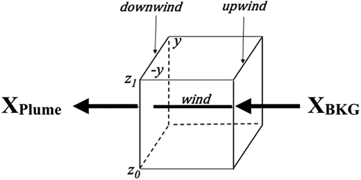
Schematic representation of the mass balance approach for determining top-down emission rates. DOI: https://doi.org/10.1525/elementa.2020.121.f4
Schematic representation of the mass balance approach for determining top-down emission rates. DOI: https://doi.org/10.1525/elementa.2020.121.f4
In this equation, v (m/s) is the wind velocity and cos(θ) is the angle (in radians) between the normal to the aircraft heading and the wind direction (WND), the values for which are taken from the aircraft inertial navigation system and will be further discussed. Since the resulting cos(θ) angle term is constantly changing over the plume width (to be discussed), it cannot be removed from the double integral as a constant. The term Nair represents the ideal gas law moles of air in m−3, for the specific measured plume air temperature and pressure. The crosswind plume length from –y to y was determined for each 1-s plume measurement period employing the aircraft speed. The term (XPlume − XBkg) represents the measured difference between the plume mixing ratio and a constant background inflow value in units of ppbv for each of the 33 VOCs tabulated in Table 1 plus the six continuous measurements. Each mixing ratio difference is multiplied by 1 × 10⁻⁹ and the individual molecular weights (Mw, g/mole). These terms when integrated over the plume crosswind dimensions from –y to +y in meters and over the plume depth from the surface at z0 to the maximum height at z1 in meters, with the assumption that the emissions fill the entire mixed layer depth (MLD), one arrives at emission rates E (g/s) for each of the 33 VOCs plus the six continuous measurements. Here, z1 accounts for the top of the planetary layer plus a portion of the entrainment zone, as in Peischl et al. (2015). This will be further discussed in Section 5.3.
In contrast to previous mass balance studies, where the flight patterns were specifically designed to sample upwind and downwind walls in straight line headings normal to the wind vectors surrounding the regions of interest at different altitudes, in this study, the DC8 intercepted Daesan plumes in curved paths which were sampled in a limited altitude range. This, and the fact that most of the VOC measurements of this study were acquired by integrative WAS sampling, presents some challenges when determining top-down VOC emission rates employing the mass balance approach. Despite these challenges, in this study, we show that with careful analysis of each term in the mass balance equation, one can derive top-down emission rate estimates for VOCs, CH2O as well as its precursors from the Daesan facility within conservative estimated uncertainty bounds derived from analysis of each term. This was carried out for five individual emission plumes spanning 3 days, 2 weekday and 1 weekend period in June 2016, and the results were extrapolated to yearly Daesan emission estimates and compared to bottom-up yearly inventory estimates. The following sections will address each of these challenges and the approaches employed.
5.1. Identification of upwind and downwind flight legs employed and determination of WAS correction factors
The most important challenge is the identification of upwind and downwind flight legs appropriate for the mass balance approach. Not only is this important for this study, it is germane for all other studies where top-down flux estimates are determined, employing integrative sampling approaches. As mentioned, the WAS system provides integrative VOC measurements acquired over discrete sampling intervals typically in the 34–37 s range. During KORUS-AQ, it was not possible to precisely time the WAS sampling intervals to exactly match the full plume time intervals, and this can be seen in Figure 5A. Here we show time series measurements for midmorning plumes on June 5, 2016. The plume extents, shown by the dark rectangles for Plumes 1 and 3, were determined by the temporal profiles of the six continuous measurements and their sharp concentration gradients at both plume edges. Figure 5A shows the temporal profiles for four of these continuous measurements (CH2O, C2H6, benzene, and toluene) by continuous lines, and Figure 5B shows this for continuous 1-s measurements of SO2 and CO. These fast measurements were shifted in time as necessary, typically by 1–2 s, to co-align sharp features in order to remove small residual instrumental time lags. Figure 5A also shows the discrete WAS measurements of ethane, benzene, and toluene as crosses (which in all figures throughout appear as solid horizontal bars) the temporal bounds for which are highlighted by the light cross-hatched rectangles. All-time series of this study will be presented in this same format. It is important to note that all 33 WAS VOC compounds employed in our mass balance approach were acquired in these same discrete sampling periods. As can be seen, Plume 3 contains two WAS sampling segments, labeled A and B, while Plume 1 contains one segment. As we will show, Daesan plumes on June 2 and June 3 each contained two WAS sampling segments.
![(A) June 5, 2016 time series around the Daesan petrochemical complex at an altitude around 300 m for 1-s DC-8 measurements of compact airborne multispecies spectrometer (CAMS) CH2O (blue line), CAMS C2H6 (red line), proton transfer reaction mass spectrometry (PTRMS) benzene (black dotted line), PTRMS toluene (green dotted line) along with integrative whole air sampler (WAS) ethane (red crosses), benzene (black crosses), and toluene (green crosses). The WAS crosses in all cases appear as solid horizontal bars. Downwind Plumes 1 and 3 are shown along with inflow time periods from two different time periods (Original Bkg and an Alternative Bkg). Figure 5C displays these time periods on a map with the Daesan complex. The mass balance downwind sampling periods for the continuous measurements are shown in the dark gray rectangles, while the light cross-hatched periods within these intervals designate the WAS sampling periods used in this analysis. (B) Same time series as Figure 5A showing in addition continuous 1-s SO2 measurements from the Georgia Institute of Technology chemical ionization mass spectrometric instrument (black line) and CO (gray line) from differential absorption carbon monoxide. (C) Flight tracks at altitudes around 300 m in the morning around 10:50 (local) around the Daesan complex on June 5, 2016. The flight legs are colored and sized by the CH2O concentrations measured on the DC-8. Wind vectors (direction and wind speed times 10 for emphasis) acquired by the DC-8 inertial navigation system are displayed by the red arrows on every third point. As shown in Figure S1, some of these vectors yield erroneous information, as they are affected by aircraft heading and roll, especially in tight turns. The latest Daesan bottom-up VOC emission inventory (from Konkuk University [KORUSv5] emission inventory) is displayed in this figure by the filled black circles, which are sized by their emission rates in MT/year, the largest of which is highlighted. The text further discusses the plume outflow and inflow extents. DOI: https://doi.org/10.1525/elementa.2020.121.f5](https://ucp.silverchair-cdn.com/ucp/content_public/journal/elementa/8/1/10.1525_elementa.2020.121/3/m_elementa.2020.121.f05a.png?Expires=1716292690&Signature=Qc3abVRNNAXcFMunyx2rBL7AyXVC9aLzcXmsjAOnyiSKGqT3r9Z2La2oBIJ6Za9YtA8xs0qmtJ0benfLS0OtHOdHclYrpJXQPMnJusdRs4BYNqHrDiodOT-SfUMAZ3nliXgowG6nV3rQmm8YUrELn9TdOG0c5s3Gtizwa6QM9EsD~m5Y8M9B00kVf3KTsuqgnsQ15UWkURTpXXbXAmreht~uamJezxePqlyvz9yNUI8r1qbWKdFp6e2PcP~~1vzQFCyhXaVJ0LFwben1nOzkfz1pftioDU-fGM4wUgCBQDIa3lYX-rcaC-AUurdld6OlN6~Dt9GHImqd9jxM169UjQ__&Key-Pair-Id=APKAIE5G5CRDK6RD3PGA)
![(A) June 5, 2016 time series around the Daesan petrochemical complex at an altitude around 300 m for 1-s DC-8 measurements of compact airborne multispecies spectrometer (CAMS) CH2O (blue line), CAMS C2H6 (red line), proton transfer reaction mass spectrometry (PTRMS) benzene (black dotted line), PTRMS toluene (green dotted line) along with integrative whole air sampler (WAS) ethane (red crosses), benzene (black crosses), and toluene (green crosses). The WAS crosses in all cases appear as solid horizontal bars. Downwind Plumes 1 and 3 are shown along with inflow time periods from two different time periods (Original Bkg and an Alternative Bkg). Figure 5C displays these time periods on a map with the Daesan complex. The mass balance downwind sampling periods for the continuous measurements are shown in the dark gray rectangles, while the light cross-hatched periods within these intervals designate the WAS sampling periods used in this analysis. (B) Same time series as Figure 5A showing in addition continuous 1-s SO2 measurements from the Georgia Institute of Technology chemical ionization mass spectrometric instrument (black line) and CO (gray line) from differential absorption carbon monoxide. (C) Flight tracks at altitudes around 300 m in the morning around 10:50 (local) around the Daesan complex on June 5, 2016. The flight legs are colored and sized by the CH2O concentrations measured on the DC-8. Wind vectors (direction and wind speed times 10 for emphasis) acquired by the DC-8 inertial navigation system are displayed by the red arrows on every third point. As shown in Figure S1, some of these vectors yield erroneous information, as they are affected by aircraft heading and roll, especially in tight turns. The latest Daesan bottom-up VOC emission inventory (from Konkuk University [KORUSv5] emission inventory) is displayed in this figure by the filled black circles, which are sized by their emission rates in MT/year, the largest of which is highlighted. The text further discusses the plume outflow and inflow extents. DOI: https://doi.org/10.1525/elementa.2020.121.f5](https://ucp.silverchair-cdn.com/ucp/content_public/journal/elementa/8/1/10.1525_elementa.2020.121/3/m_elementa.2020.121.f05b.png?Expires=1716292690&Signature=p53Nr0edqGZ3vdiUkWGJhhl9l4YruiWasrc-qtcW61JUHmdQcIiRrJuQR-VX3cqep5wrUp9p9vFAFmTXWLbv~Z~wL1nIx6TqsIQW-osfc5TP~oCP4BMz0QX3Hp2M6JdPH7dMqSre25jk82b2nOn2896-TAg85lsM-FxqPE0kjvXsC3QUkltvRlNz745~OtZEHNFwRRHZy0N-inq2T3p5~WHIRfV8RVHjXBiwJrICEk9LoZM1T73ac5cRPN6LHEszcFSMvfL6xzE0SYJIdHMB5AhMbLSoGgb5T4tmYG2AZECH3HXoHsMhNTZR6Cm2M1NxFEwmzyall8xtVowSOw5vOQ__&Key-Pair-Id=APKAIE5G5CRDK6RD3PGA)
(A) June 5, 2016 time series around the Daesan petrochemical complex at an altitude around 300 m for 1-s DC-8 measurements of compact airborne multispecies spectrometer (CAMS) CH2O (blue line), CAMS C2H6 (red line), proton transfer reaction mass spectrometry (PTRMS) benzene (black dotted line), PTRMS toluene (green dotted line) along with integrative whole air sampler (WAS) ethane (red crosses), benzene (black crosses), and toluene (green crosses). The WAS crosses in all cases appear as solid horizontal bars. Downwind Plumes 1 and 3 are shown along with inflow time periods from two different time periods (Original Bkg and an Alternative Bkg). Figure 5C displays these time periods on a map with the Daesan complex. The mass balance downwind sampling periods for the continuous measurements are shown in the dark gray rectangles, while the light cross-hatched periods within these intervals designate the WAS sampling periods used in this analysis. (B) Same time series as Figure 5A showing in addition continuous 1-s SO2 measurements from the Georgia Institute of Technology chemical ionization mass spectrometric instrument (black line) and CO (gray line) from differential absorption carbon monoxide. (C) Flight tracks at altitudes around 300 m in the morning around 10:50 (local) around the Daesan complex on June 5, 2016. The flight legs are colored and sized by the CH2O concentrations measured on the DC-8. Wind vectors (direction and wind speed times 10 for emphasis) acquired by the DC-8 inertial navigation system are displayed by the red arrows on every third point. As shown in Figure S1, some of these vectors yield erroneous information, as they are affected by aircraft heading and roll, especially in tight turns. The latest Daesan bottom-up VOC emission inventory (from Konkuk University [KORUSv5] emission inventory) is displayed in this figure by the filled black circles, which are sized by their emission rates in MT/year, the largest of which is highlighted. The text further discusses the plume outflow and inflow extents. DOI: https://doi.org/10.1525/elementa.2020.121.f5
(A) June 5, 2016 time series around the Daesan petrochemical complex at an altitude around 300 m for 1-s DC-8 measurements of compact airborne multispecies spectrometer (CAMS) CH2O (blue line), CAMS C2H6 (red line), proton transfer reaction mass spectrometry (PTRMS) benzene (black dotted line), PTRMS toluene (green dotted line) along with integrative whole air sampler (WAS) ethane (red crosses), benzene (black crosses), and toluene (green crosses). The WAS crosses in all cases appear as solid horizontal bars. Downwind Plumes 1 and 3 are shown along with inflow time periods from two different time periods (Original Bkg and an Alternative Bkg). Figure 5C displays these time periods on a map with the Daesan complex. The mass balance downwind sampling periods for the continuous measurements are shown in the dark gray rectangles, while the light cross-hatched periods within these intervals designate the WAS sampling periods used in this analysis. (B) Same time series as Figure 5A showing in addition continuous 1-s SO2 measurements from the Georgia Institute of Technology chemical ionization mass spectrometric instrument (black line) and CO (gray line) from differential absorption carbon monoxide. (C) Flight tracks at altitudes around 300 m in the morning around 10:50 (local) around the Daesan complex on June 5, 2016. The flight legs are colored and sized by the CH2O concentrations measured on the DC-8. Wind vectors (direction and wind speed times 10 for emphasis) acquired by the DC-8 inertial navigation system are displayed by the red arrows on every third point. As shown in Figure S1, some of these vectors yield erroneous information, as they are affected by aircraft heading and roll, especially in tight turns. The latest Daesan bottom-up VOC emission inventory (from Konkuk University [KORUSv5] emission inventory) is displayed in this figure by the filled black circles, which are sized by their emission rates in MT/year, the largest of which is highlighted. The text further discusses the plume outflow and inflow extents. DOI: https://doi.org/10.1525/elementa.2020.121.f5
Each of the WAS sampling segments was treated independently for each of the 33 VOC compounds. Referring to Plume 3 of Figure 5A, the WAS sampling segments A and B reveal significant missing elevated plume sections and at the same time additional lower level sections outside the plume boundaries. Thus, relying on simple WAS averages of the pertinent segments could result in systematic VOC errors in both directions. To account for these effects, we determine multiplicative correction factors (CFs) for each plume by comparing the emission factors from Equation 1 for the six continuous measurements (CH2O, C2H6, benzene, toluene, SO2, and CO) integrated over the full plume width (Ei, Full Plume, dark rectangles) relative to the emission factors for these same six measurements summed over each of the individual flight segments (Seg. A and Seg. B for Plume 3 in this case) defined by the WAS sampling periods (Ei, SegA, Ei, SegB, crosshatched periods). These six continuous measurements reflect both Daesan combustion processes and fugitive emissions. Treating the WAS sampling periods as distinct periods relies on the additive property of integrals (i.e., the and treats the six continuous measurements on the WAS sampling intervals over the full plume width. In this process, we compare measurements from the same instrument over the different periods rather than a comparison of continuous measurements with the integrative WAS measurements to avoid potential complications from nonlinear WAS sampling (i.e., faster WAS measurements acquired early in the fill compared to later, which could yield erroneous results during large concentration changes). As shown in Equation 2, the average value of the ratio determines the CF, and the individual contributions and resultant average are tabulated in Table 4. We note that each plume has a different CF since the WAS coverage was different in each plume. The CF for Plume 1 with only one WAS segment was determined in a similar fashion by comparing the full plume emissions to that for Segment A. Here the small WAS segment at around 10:55 was not included since it encompasses less than 7% of the total plume area shown by the dark plume bounds and thus has the majority of its contribution outside the plume.
Correction factors (CFs) employed in the analysis of individual plumes based upon 1 s continuous measurements. DOI: https://doi.org/10.1525/elementa.2020.121.t4
| Day Date Plume No. | CH2O | C2H6 | Benzene | Toluene | SO2 | CO | Average |
|---|---|---|---|---|---|---|---|
| Thursday June 2, 2016, Plume 4 | 2.46 | 2.23 | 1.99 | 2.16 | 2.29 | 2.09 | 2.2 ± 0.16 (0.074) |
| Friday June 3, 2016, Plume 3 | 2.66 | 2.30 | 2.80 | 2.42 | 2.31 | 2.5 ± 0.22 (0.089) | |
| Friday June 3, 2016, Plume 4 | 1.41 | 1.40 | 1.37 | 1.43 | 1.30 | 1.32 | 1.4 ± 0.061 (0.044) |
| Sunday June 6, 2016, Plume 1 | 1.22 | 1.20 | 1.19 | 1.16 | 1.25 | 1.23 | 1.2 ± 0.032 (0.026) |
| Sunday June 5, 2016, Plume 3 | 1.14 | 1.32 | 1.09 | 1.07 | 1.40 | 1.13 | 1.2 ± 0.13 (0.11) |
The two bold-faced values highlight large differences with the other CFs. The last column lists the average, the standard deviation and the relative standard deviation (σ/mean) in parenthesis. All values in the last column have been rounded to two significant figures.
These correction factors are then multiplied by the sum of the WAS VOC flux estimates determined for each plume segment to arrive at a total VOC and individual VOC emission rate (g/s) in accordance with Equation 3:
As can be seen in Table 4, the individual CF components yield remarkable consistency for some plumes (e.g., Plume 1 on June 5) as well as large differences that are highlighted in bold for some of the components (namely C2H6 and SO2). As can be seen by these CFs, not accounting for such corrections in the current study can result in a low bias for the top-down VOC estimates ranging from a factor of 1.2 to 2.5.
Figure 5C displays midmorning (10:50 local time) DC-8 flight tracks around the Daesan complex on June 5, 2016, superimposed on the Daesan facility bounds in the shaded region. The largest Daesan emission source is indicated by the largest filled circle and highlighted by the text callout. This source is comprised of a number of individual sources at the same location (36.996°N latitude, 126.407° longitude) and has a combined VOC inventory emission rate 4,709 MT/year. All Daesan emission plots employ this same VOC inventory scale. Figure 5C also displays wind vectors acquired by the DC-8 inertial navigation system. As will be discussed in Section 5.2, some of these vectors yield erroneous information, as they are affected by aircraft heading and roll, especially in tight turns. An average wind direction and wind speed (71° ± 14°, 4.5 ± 0.7 m/s, designated by the large black arrow) for this entire sampling period was determined based on select time periods where the aircraft motion had minimal impact on the derived winds. Figure 5C shows three distinct Daesan outflow plumes. Plumes 1 and 2 intercept outflow immediately over the western portion of the Daesan complex, whereas the maximum CH2O outflow in Plume 3 intercepted a plume slightly downwind (approximately 1.8 km from the maximum CH2O location over Daesan) and approximately 7.1 km from the maximum Daesan VOC emission source.
Plumes 1 and 3 are the same plumes depicted in Figure 5A, and both plumes are further analyzed here. Plume 2 was excluded since the aircraft heading dramatically changed during this flight leg in passing right over the Daesan complex resulting in a heading that was no longer normal to the wind direction. The downwind plume extents identified in Figure 5A are displayed by the O symbols in Figure 5C along with the upwind inflow plume extents by the red O symbols, which are designated in Figure 5A by the “Original Bkg” label. Each of the five plumes of this study spanning three individual flight days will be displayed in the same format as Figure 5A and C. We also display in Figure 5C an alternative inflow background period by the red □ symbols and designated by the label “Alternative Bkg” in Figure 5A and B. Although it is clear from five of the six continuous tracers that this alternative background period is contaminated by elevated measurements, and hence is not a good background choice, we present VOC flux calculations here to show the relative insensitivity of our calculations to the optimum choice of inflow period. This arises from the fact that the Daesan plume emissions are large compared to species concentrations along the sides of this facility that are not directly in the plume outflow path.
Perhaps a bigger challenge in our analysis is the identification of downwind flight legs that are far enough downwind to represent a well-mixed plume in vertical and horizontal directions emanating from all the Daesan facility emission sources and whose leg length captures the entire plume and yet close enough to where other emission sources (e.g., other facilities and/or local ship plumes over the Yellow Sea) can be eliminated. This challenge arises because the Daesan complex is comprised of at least 18 separate plants involving different processing and spanning a very large area. This results in plume heterogeneity, which is further complicated by the fact that this study does not have the exact location of the emission sources sampled by the DC-8 for each plume. This will be further discussed in Section 6.1.
5.2. Determination of appropriate DC-8 wind vectors to employ
Equation 1 shows the importance of accurate wind vectors (direction and speed) in the accuracy of top-down emission estimates employing the mass balance approach. The wind speed linearly affects the results, while the wind direction affects the results nonlinearly through the cos(θ) term. As stated, the DC-8 inertial navigation wind vectors can be affected by aircraft heading and roll maneuvers, especially in tight turns. A careful inspection of Figure 5C reveals that the displayed instantaneous wind vectors in some cases erroneously follow the aircraft heading in tight turns, and Figure S1 and the associated discussion further illustrate this point. To minimize these effects, we have identified straight and level flight legs as well as periods where the aircraft heading does not undergo large discontinuities (i.e., tight turns), and changes in roll angle are kept to a minimum in the determination of wind vectors. In all cases, we support these determinations of wind direction, wind speed, and the constancy of both employing multiple Flexible Particle dispersion model (FLEXPART) back trajectories using National Centers for Environmental Prediction Global Forecast System analysis over the regions of interest, which encompasses the inflow and outflow periods.
5.3. Estimates of MLD and its uniformity
Like wind direction and speed, the mass balance approach of Equation 1 relies on an accurate knowledge of the MLD as well as evidence that the Daesan emissions fill the entire MLD. Following the analysis of Peischl et al. (2015), the MLD was modified to include mixing in the entrainment zone, which results in a Z1 value defined by Peischl in Equation 4:
Here ZPBL is the PBL and Ze is the top of the entrainment zone. Figure 6A shows vertical profiles of CO, C2H6, CH2O, CH4, and CO2 acquired during an en route vertical descent on the way in to Daesan. Unlike these five gases, profiles of temperature, potential temperature, and equivalent potential temperature were too noisy to clearly discern ZPBL and Ze. The dashed black lines visually indicate a ZPBL radar altitude of 0.58 km and a Ze of 0.63 km, which from Equation 4 yields Z1 = 0.59 km. The DC-8 location where the vertical profile was acquired was slightly south of Daesan and is highlighted by the circle labeled Profile in the lower right panel Figure 6B. Fortunately, aerosol backscatter lidar measurements from the NASA Langley Research Center airborne HSRL on the DC-8 were also available and allowed us to further verify the results of Figure 6A directly in the Daesan Plumes 1 and 3 displayed in Figure 5A–C. Equation 4 was employed in determining the MLD Z1. Despite the fact that only in one case (dark blue trace in upper left panel) we clearly observe the top of the PBL, further inspection of the actual HSRL images indicates that our estimates for all other traces are very close to this same PBL altitude. At the Profile location shown in the lower right panel, this resulted in a Z1 = 0.59 km, which is identical to that in Figure 6A. Based upon the spread in HSRL-determined values and the comparison with the chemical species, we estimate a 1σ uncertainty of ± 0.05 km for the June 5 plume cases. The June 2 plume case likewise resulted in an MLD of 0.59 km from HSRL and 0.58 km from the in situ profiles and an estimate of ±0.05 km for the uncertainty. The plumes on June 3 were slightly more complicated to analyze since the DC-8 was flying slightly higher, resulting in greater ambiguity in the ZPBL determinations, and the in situ profiles were acquired over the SMA area approximately 67 km away from Daesan as opposed to the HSRL profiles obtained approximately 7 km away. The HSRL measurements nevertheless provide bounds (ZPBL 0.66 km, and Ze 0.78–0.83 km) from which we estimate an MLD of 0.70 km with a larger assigned uncertainty of ±0.1 km. These HSRL-determined MLDs and uncertainty limits employed in our analysis are tabulated in Table 5 in our discussions of individual plumes.

(A) Radar altitude profiles on June 5 for local times of 10:37–10:54 upstream of Daesan. The five chemical species indicate a ZPBL of 0.58 km and the top of the entrainment zone height (Ze) of 0.63 km, resulting in a Z1 value of 0.59 km. See the manuscript for the definition of these terms. These values were visually estimated by the sharp gradients in the various chemical species. (B) High spectral resolution lidar backscatter ratio values acquired on June 5 (top traces) and the map location where each backscatter was acquired relative to Daesan (shown by the shaded region next to the coast). The panels on the right are for Plume 3 and on the left are for Plume 1 on June 5. The aircraft flight altitudes (Flt Alt.) are indicated by the black points connected by lines. The dashed lines indicate the extrapolation from the top of the PBL to the top of the entrainment zone (EZ, Ze in Equation 4), with the EZ values estimated by a change in curvature in the backscatter ratios. PBL = planetary boundary layer. DOI: https://doi.org/10.1525/elementa.2020.121.f6
(A) Radar altitude profiles on June 5 for local times of 10:37–10:54 upstream of Daesan. The five chemical species indicate a ZPBL of 0.58 km and the top of the entrainment zone height (Ze) of 0.63 km, resulting in a Z1 value of 0.59 km. See the manuscript for the definition of these terms. These values were visually estimated by the sharp gradients in the various chemical species. (B) High spectral resolution lidar backscatter ratio values acquired on June 5 (top traces) and the map location where each backscatter was acquired relative to Daesan (shown by the shaded region next to the coast). The panels on the right are for Plume 3 and on the left are for Plume 1 on June 5. The aircraft flight altitudes (Flt Alt.) are indicated by the black points connected by lines. The dashed lines indicate the extrapolation from the top of the PBL to the top of the entrainment zone (EZ, Ze in Equation 4), with the EZ values estimated by a change in curvature in the backscatter ratios. PBL = planetary boundary layer. DOI: https://doi.org/10.1525/elementa.2020.121.f6
Terms used in the calculation of flux (Equation 1) and fractional uncertainties in (σ/mean value) in parentheses. DOI: https://doi.org/10.1525/elementa.2020.121.t5
| Day Date Plume No. | Time Start | Time Stop | v (m/s) | Cos(θ) | Z1 MLD (km) | N (moles/m3) | L (km) | Average CF |
|---|---|---|---|---|---|---|---|---|
| Thursday June 2, 2016, Plume 4 | 11:41:41 | 11:43:50 | 2.7 (0.49) | 0.76 (0.12) | 0.59 (0.09) | 40 (0.001) | 15 (0.008) | 2.2 (0.074) |
| Friday June 3, 2016, Plume 3 | 11:34:20 | 11:35:45 | 2.2 (0.45) | 0.78 (0.18) | 0.70 (0.14) | 40 (0.001) | 11 (0.01) | 2.5 (0.089) |
| Friday June 3, 2016, Plume 4 | 11:39:45 | 11:41:09 | 2.2 (0.45) | 0.86 (0.06) | 0.70 (0.14) | 40 (0.001) | 11 (0.01) | 1.4 (0.044) |
| Sunday June 5, 2016, Plume 1 | 10:54:03 | 10:54:59 | 4.5 (0.27) | 0.85 (0.20) | 0.59 (0.09) | 40 (0.001) | 5.7 (0.03) | 1.2 (0.026) |
| Sunday June 5, 2016, Plume 3 | 10:49:16 | 10:50:31 | 4.5 (0.27) | 0.86 (0.15) | 0.59 (0.09) | 40 (0.001) | 8.9 (0.01) | 1.2 (0.11) |
All times and dates are all local and represent the full downwind plume intercept times based upon the fast measurements. The mixed layer depth (Z1, MLD) was determined from high spectral resolution lidar backscatter measurements using Equation 4 and estimates of the planetary boundary layer and the top of the entrainment zone. The terms v (m/s) and cos(θ) are the wind velocity and the angle between the normal to the aircraft heading and the wind direction, respectively. The term Nair represents the ideal gas law moles of air in m−3, and the term L represents the crosswind plume length in km. The CF term is a correction factor applied to whole air sampler measurements (see Section 5.1). All parameters listed have been rounded to two significant figures, but the full unrounded values are used in the calculations in the double integrals of Equation 1. The June 2 Plume 4 values reflect the full plume as discussed in Section 6.2.
Just as important as the mixed layer height is an assessment that the Daesan emissions uniformly fill the entire mixed layer from the surface to the mixed layer height. We believe this to be the case since the emissions are not isolated events in time but result from continuous emissions over the course of many days of facility operations. Daesan plume intercepts on June 3 verify uniform mixing from the surface up to at least 0.43 km, which comprises at least 61% of the MLD of 0.70 km on this day. Additional details of this analysis can be found in Figures S2 and S3 along with the associated discussions in the Supplement. Section 7.1, where we show comparisons of the bottom-up Daesan SO2 emission inventory based upon continuous in-stack measurements with top-down estimates from our mass balance approach assuming that the Daesan emissions fill the entire MLD, will provide additional supporting evidence.
5.4. Estimation of a lower limit for PC-produced CH2O from Daesan
As stated, CH2O is both directly emitted and PC produced in petrochemical plumes. In some cases, the production of CH2O from ethene and propene emissions, and especially 1,3-butadiene and styrene, is so fast that the distinction between emission and production becomes blurred. Nevertheless, it is important to separate out these two sources of CH2O. Since CH2O only has a midday lifetime of approximately 2–3 h, CH2O levels of approximately 34 ppb observed (to be shown for June 2 plume) approximately 6.6 km downwind of the maximum Daesan VOC emission source, if directly emitted, would yield levels less than approximately 5 ppb by the time the Daesan airmass reached the SMA. This is based upon a travel distance of approximately 80 km and typical prevailing average wind speeds of 13 km/h observed at the Gimpo airport in July over the time period of 2009–2016. However, PC-produced CH2O from its two primary petrochemical sources, ethene and propene, could significantly extend its influence footprint. Photochemical ethene emissions, for example, with a lifetime in the 3–8 h range (Wert et al., 2003, for OH levels of 1 × 10⁷ to 4 × 10⁶ molecules/cm−3) would significantly extend downwind CH2O concentrations. In this case, Daesan emissions could have a significant effect on the SMA at times in July and potentially at times for other months. In addition, under light wind conditions, PC-produced CH2O could also impact regions in close proximity to Daesan, as will be shown. Hence, one goal of this study is to assess this lower limit for PC-produced CH2O from the various Daesan plumes. We accomplish this employing the CIT CIMS measurements of AHNs, as discussed by Teng et al. (2015).
In Teng et al. (2015), the OH oxidation of alkenes proceeds via two paths (see Figure S4 and Table S2): a primary path where OH and O2 add across the double bond followed by O extraction from NO to produce various aldehydes (lower path) and NO2 and a minor path (upper path) where NO is added to produce hydroxynitrates. In contrast to the major path, the hydroxynitrates from the minor path are only produced by secondary photochemistry and not directly emitted. Therefore, the CIT AHN measurements in conjunction with a knowledge of the oxidation branching ratio (α) and the CH2O quantum yield (γ) can be used in the assessment of PC-produced CH2O. As indicated in Figure S4, the sum in Equation 5 of the AHN measured by the CIT CIMS instrument provides a lower limit to PC-produced CH2O via
The AHNs, their CH2O quantum yields, and their branching ratios, which are taken from Teng et al. (2015), are reproduced in Table S2. A sixth AHN from styrene was estimated from the ratio of the WAS [styrene]/[1,3-budadiene] × the WAS [1,3-butadiene], and this also was included in the sum. All plots and discussions of PC-produced CH2O employing Equation 5 are henceforth referred to as [CH2O]PC. These are lower limits since only six AHN are included in this analysis, and some of the oxidation products like 1,3-butadiene are highly reactive and most likely represent lower limits from the CIT CIMS instrument.
In our analysis of top-down Daesan emission fluxes, we therefore account for PC-produced CH2O from the following. Like the VOC emission fluxes, we determine the difference in PC-produced CH2O from the AHN sum between the downwind and upwind legs (Δ[CH2O]PC). Equation 6 yields an upper limit for directly emitted CH2O via
Here the difference between downwind and upwind CH2O values is obtained from the CAMS CH2O measurements. This is an upper limit since as discussed, the AHN sum represents a lower limit to PC-produced CH2O. Figure S5 and the associated discussion provides an example of the resulting linear correlations between [CH2O]PC and measured CH2O from the CAMS instrument for the June 2, 2016, Daesan plumes. Figure S5 shows nearly identical slopes around 63% for the lower limit of PC-produced CH2O spanning both the entire Daesan sampling region shown in Figure S9 (to be discussed) and measurements directly over Daesan. Hence, the air quality over and around Daesan is highly processed. For facility of discussion, throughout the rest of this article, we refer to the derived slope from this linear regression relationship as the AHN-CH2O slope.
6. Analysis of top-down VOC Daesan emissions for individual plumes and total uncertainty estimates
We analyzed five individual midmorning Daesan plumes employing the procedures discussed above, and these include one plume on Thursday June 2 (with two different outflow limits), two plumes on Friday June 3, and two plumes on Sunday June 5. The local plume times and dates are tabulated in Table 5 along with six of the seven terms employed in our analysis employing Equation 1. The seventh term is the measured difference between plume outflow mixing ratio and the background inflow value for each of the species analyzed. The values listed in Table 5 are the plume-averaged values, and we show these terms and their fractional uncertainties (1σ/mean) in the parenthesis in order to compare the component uncertainties that comprise the total uncertainty. It is important to note that our calculation for each emission rate from Equation 1 actually employs the instantaneous values measured in 1-s increments across each plume and evaluated by the double integral and not simply the multiplication of these plume-averaged terms. As discussed previously, the wind speed, wind direction, mixed layer height, and background inflow mixing ratios are constants in these determinations, and the variables of integration are the cos(θ), N (moles/m3), plume length (km, from the aircraft speed × plume width in seconds), the averaged CF, and the instantaneous plume outflow mixing ratios. The systematic uncertainty estimates for the DC-8 measurement probes listed in Table S1 were employed here. In the case of the CF, the uncertainty is based upon the standard deviation of the average for the six fast tracers given in Table 4. The uncertainty in the delta mixing ratios for each constituent was derived from the values listed in Table 1. We do not include uncertainties in the AHN in this analysis of CH2O emissions since these measurements yield an upper limit for the emitted CH2O, and we are unable to quantify this factor. As can be seen, the uncertainty in the wind speed measurement, which is comprised of the imprecision in its determination from the various appropriate flight legs added in quadrature to the ±1 m/s systematic term, in all cases yields the largest contribution to the total uncertainty. We note, however, that based upon comparisons with wind speeds derived from FLEXPART back trajectories, the total uncertainty estimates for the June 2 and June 3 wind speeds are too conservative: FLEXPART-derived wind speeds here are within 3% of the determined values listed in Table 5. In the case of June 5, the listed uncertainty estimates are more in line with FLEXPART comparisons, which yield wind speeds 24% lower. Our mass balance uncertainty estimates in all cases employ the values tabulated in Table 5.
The second largest uncertainty term listed in Table 5 is the cos(θ) term. To evaluate the uncertainty in the cos(θ) term, we calculated the average plume value for this term employing the instantaneous aircraft heading at each 1-s interval (HDGi) the normal to the fixed wind direction WNDn using the value determined described in Section 5.2. The average value of cos(θ) is determined across the entire plume width from –y to y in Equation 7, where n is the number of measurements:
We repeat this calculation two more times, substituting the following values in place of WNDn to reflect upper limit (UL) and lower limit (LL) to the wind direction normal:
The wind direction uncertainty is thus comprised of the imprecision in its determination (σimp) and its systematic value (σsys) from Table S1. This produces a UL and LL for the average cos(θ) term, which because of the nonlinear cos term is asymmetric about the mean plume value. For facility in our calculations, we conservatively take the larger of the two differences from the mean to reflect the total uncertainty estimate (σtotal) in the cos(θ) term, and Table 5 lists the mean value and a conservative UL for the fractional uncertainty (σtotal/mean) from this analysis.
Table 6 lists the rounded instantaneous emission rates (g/s), while Table 7 tabulates the yearly emission rate estimates (MT/year) using Equation 8 for comparisons with the bottom-up emission inventories. This table also includes the yearly estimates for CH2O emissions plus its four major precursors (ethene, propene, 1,3-butadiene, and 1-butene) calculated in the same manner as the VOCs. We note that these four major CH2O precursors are also included in the VOC emissions category.
Instantaneous Daesan emission fluxes E (g/s) from the double integration of Equation 1 for each of the 33 WAS VOCs compounds for each of the five plumes of this study, plus CH2O and SO2. DOI: https://doi.org/10.1525/elementa.2020.121.t6
| WAS VOCs | June 2 Plume 4 | June 3 Plume 3 | June 3 Plume 4 | June 5 Plume 1 | June 5 Plume 3 | Average of Five Plumes | Top 10 Rank Values |
|---|---|---|---|---|---|---|---|
| 1. Ethane | 48 | 34 | 44 | 58 | 53 | 47 | |
| 2. Propane | 114 | 256 | 375 | 124 | 108 | 195 | 3 |
| 3. i-Butane | 240 | 78 | 75 | 146 | 114 | 131 | 5 |
| 4. n-Butane | 167 | 79 | 88 | 124 | 113 | 114 | 7 |
| 5. i-Pentane | 101 | 73 | 91 | 92 | 106 | 93 | 9 |
| 6. n-Pentane | 61 | 63 | 74 | 55 | 62 | 63 | 12 |
| 7. n-Hexane | 195 | 192 | 178 | 397 | 202 | 233 | 2 |
| 8. n-Heptane | 11 | 13 | 11 | 22 | 17 | 15 | |
| 9. n-Octane | 7 | 7 | 6 | 24 | 13 | 11 | |
| 10. n-Nonane | 3 | 3 | 2 | 8 | 7 | 5 | |
| 11. n-Decane | 5 | 2 | 3 | 12 | 5 | 5 | |
| 12. 2,3-Dimethylbutane | 14 | 10 | 10 | 24 | 13 | 14 | |
| 13. 2-Methylpentane | 54 | 40 | 49 | 110 | 57 | 62 | |
| 14. 3-Methylpentane | 100 | 93 | 95 | 232 | 117 | 127 | 6 |
| 15. Cyclopentane | 7 | 6 | 8 | 6 | 8 | 7 | |
| 16. Methylcyclopentane | 66 | 44 | 43 | 76 | 49 | 56 | |
| 17. Cyclohexane | 39 | 12 | 16 | 29 | 12 | 22 | |
| 18. Methylcyclohexane | 5 | 5 | 5 | 8 | 7 | 6 | |
| 19. Ethene | 367 | 138 | 174 | 352 | 251 | 257 | 1 |
| 20. Propene | 147 | 38 | 55 | 171 | 93 | 101 | 8 |
| 21. 1-Butene | 18 | 3 | 4 | 31 | 15 | 14 | |
| 22. i-Butene | 12 | Nan | 14 | Nan | Nan | 13 | |
| 23. cis-2-Butene | 1 | 0.4 | 0.5 | 10 | 9 | 4 | |
| 24. trans-2-Butene | 0.6 | 0.2 | 0.2 | 6 | 5 | 2 | |
| 25. 1,3-Butadiene | 26 | 3 | 1 | 100 | 44 | 35 | |
| 26. Isoprene | 3 | 6 | 4 | 7 | 6 | 5 | |
| 27. Ethyne | 13 | 4 | 4 | 13 | 10 | 9 | |
| 28. Benzene | 307 | 120 | 150 | 174 | 114 | 173 | 4 |
| 29. Toluene | 85 | 35 | 44 | 79 | 76 | 64 | 11 |
| 30. Ethylbenzene | 26 | 20 | 20 | 31 | 31 | 26 | |
| 31. m, p-Xylene | 57 | 33 | 37 | 33 | 44 | 41 | |
| 32. o-Xylene | 10 | 9 | 9 | 10 | 13 | 10 | |
| 33. Styrene | 11 | 5 | 5 | 33 | 20 | 15 | |
| Sum WAS VOCs | 2,321 | 1,421 | 1,691 | 2,601 | 1,797 | 1,966 ± 482 | |
| CAMS CH2O | 122 | 100 | 85 | 61 | 67 | 87 ± 25 | 10 |
| CH2O + Ethene + Propene + 1,3-Butadiene + 1-Butene | 680 | 281 | 317 | 716 | 471 | 493 ± 201 | |
| GIT SO2 | 655 | 373 | 330 | 355 | 361 | 415 ± 135 | |
| CH4 DACOM | 2,918 | 489 | 1,513 | 1,419 | 1,585 ± 1,002 |
The CFs tabulated in Tables 4 and 5 have been applied to the 33 WAS measurements here. The values have been rounded. The June 2 Plume 4 top-down emission fluxes are values for the full plume (see Figures S8 and S9). CFs = correction factor; WAS = whole air sampler; VOC = volatile organic compound; GIT = Georgia Institute of Technology; DACOM = differential absorption carbon monoxide measurements; CAMS = compact airborne multispecies spectrometer. The boldfaced values at the bottom of this table represent the VOC sum in the case of the WAS measurements, and in the other cases are for emphasis. Likewise, the top 10 WAS VOC rankings are boldfaced for emphasis. The uncertainties represent the Average column represents the 1σ standard deviation of the mean.
Yearly Daesan facility emission flux estimates (MT/year) for the sum of WAS VOCs (third column) and CH2O + precursors (ethene + propene + 1,3-butadiene + 1-butene) in the fourth column and SO2 in the fifth column. DOI: https://doi.org/10.1525/elementa.2020.121.t7
| Day Date | CF | (MT/Year) | Flux (CH2O + Precursors) (MT/Year) | Flux SO2 (MT/Year) |
|---|---|---|---|---|
| Thursday June 2, 2016, Plume 4 | 2.2 (0.07) | (73 ± 38) × 103 (58 ± 32) × 103 a | (21 ± 11) × 103 (18 ± 9.7) × 103 a | (21 ± 11) × 103 (13 ± 7.3) × 103 a |
| Friday June 6, 2016, Plume 3 | 2.5 (0.09) | (45 ± 23) × 103 | (8.8± 4.5) × 103 | (12 ± 6.4) × 103 |
| Friday June 3, 2026, Plume 4 | 1.4 (.04) | (53 ± 25) × 103 | (10 ± 5.0) × 103 | (10 ± 5.4) × 103 |
| Sunday June 5, 2016, Plume 1 | 1.2 (0.03) | (82 ± 29) × 103 | (23 ± 7.9) × 103 | (11 ± 4.5) × 103 |
| Sunday June 5, 2016, Plume 3 | 1.2 (0.11) | (57 ± 19) × 103 (55 ± 18) × 103 b | (15 ± 5.1) × 103 (15 ± 4.8) × 103 b | (11 ± 4.3) × 103 (10 ± 4.0) × 103 b |
All times and dates are local. The uncertainties represent the 1σ total uncertainty estimate and the CF column indicates the corrections factors discussed in Section 5.1. All flux estimates have been rounded to two significant figures.
aValues on June 2 calculated for the restricted plume for comparison with the upper values for the full plume.
bValues using the Alternative Bkg discussed in Section 6.1, which we do not recommend using. This is tabulated here to show the relative insensitivity to the proper choice of background inflow time periods.
Obviously implicit in Equation 8 is the assumption of continuous Daesan emissions, 24 h a day, 7 days a week, during all 52 weeks throughout the year. Although Daesan emissions will no doubt vary, our yearly estimates for all five plumes spanning 2 weekdays and 1 weekend are all consistently significantly higher than current bottom-up emission estimates, and thus these three sampling days to a limited extent is suggestive that the observed enhancements are not simply episodic. Such consistently enhanced VOC emissions have also been measured over Houston, TX, petrochemical facilities by Wert et al. (2003) on multiple sampling days. It is quite likely that fugitive emission sources (leakage from values, pipe connections, mechanical seals, compressors, storage tanks, etc.) make a large contribution to these petrochemical emissions in both studies. Such emissions sources, which are continuous in nature, further suggest the validity of the year-round scaling assumptions implicit in Equation 8. The validity of these assumptions is further supported by the top-down–bottom-up comparisons of SO2 emission rates in these same plumes, as will be discussed in Section 7. In the remainder of Section 6, we further discuss specifics regarding the analysis of the five plumes studied. The uncertainty estimates in Table 7 represent the total uncertainty (1σ level) in the top-down emissions determined from the quadrature addition of the systematic and random terms. As stated, these represent conservative upper limits.
6.1. Sunday June 5 midmorning Daesan Plumes 3 and 1
As indicated in Section 5.1, we analyzed Plume 3 on June 5 employing the correct background inflow period as well as an erroneous “Alternative Bkg” period to show the relative insensitivity of the results to the proper background choice in case of Daesan. The last two rows of Table 7 show the resulting (rounded) yearly top-down emission rates for the VOC sum, CH2O and its precursors, and SO2 employing the two different background inflow periods. Based on the unrounded input values in the calculations, the differences are 3%, 1%, and 9%, respectively, for the above three emission rates. This analysis shows that unless gross errors are made in the selection of the optimum background inflow periods, the derived top-down emission rates are not that sensitive to the inflow mixing ratios in the case of Daesan where the enhancements are large.
Employing the correct background period, Table 7 shows the resulting top-down emission rates for Daesan Plumes 3 and 1 studied on June 5, 2016. In this section, we present the results for a more in-depth examination of these plumes with more detailed discussions presented in the Supplement and associated Figures S6 and S7. This analysis raises the potential of missing VOC sources not captured by our mass balance determinations, and thus, the Daesan top-down results of June 5 in all likelihood represent lower emission limits. In the Supplement, we also examine the relationship between Daesan Plumes 1 and 3 on June 5. As can be seen by the results in Table 7, the derived top-down emission rates are approximately 1.5 times higher for Plume 1 compared to Plume 3 for both the VOC sum and CH2O and its four precursors, whereas the rates for SO2 are nearly equivalent in both plumes. In the Supplement, we further investigate whether differences in the source regions for the two plumes could explain these observations. This analysis, which is based on calculations for the ratio of the [AHN] to that of the parent alkene for both ethene and propene, indicates that the largest VOC emission source highlighted in Figure 5C and Figure S7 is primarily involved in both plumes. Thus, differences in the decay of the parent alkenes between the two plumes cannot explain our observations. However, because of the large heterogeneity of Daesan emissions, we cannot rule out additional contributions from other Daesan source regions to these plumes.
6.2. Thursday June 2 midmorning Daesan Plume 4
The June 2 midmorning Daesan Plume 4 time series is displayed in Figure S8, and the corresponding flight tracks on the map of the Daesan region is shown in Figure S9, in the same format as Figure 5 for June 5. As discussed in the Supplement, two different outflow limits for the upper plume extent have been identified: a narrow outflow region (hereafter referred to as restricted plume) and a more substantial outflow region (hereafter referred to as the full plume). Tables 5 and 6 present the mass balance parameters and resulting instantaneous emission values, respectively, for what we believe is the more appropriate full plume extent to analyze. For comparison purposes, Table 7 shows the yearly extrapolated results for both the full plume (upper values) and the restricted plume (lower values).
6.3. Friday June 3 midmorning Daesan Plumes 3 and 4
Plumes on this day were first discussed in Section 5.3 and in the Supplement in Figures S2 and S3 in connection with our assessment for the uniformity of the mixed layer. In this section, we further study plumes on this day in connection with the mass balance emission rates. Figure 7A, which is similar to Figure S2, displays two midmorning Daesan outflow plumes on Friday June 3. Although this figure shows multiple plumes on this day, only Plumes 3 and 4 have coincident WAS VOC measurements for analysis. The two outer rings showing Plumes 4 (next to outer ring) and 3 (outer ring) display very similar CH2O levels. As shown by the time profiles in Figure 7B, these plumes are labeled according to the intercept times. Plume 4 in Figure 7B spans the shaded region, and these are highlighted by the large open and labeled black circles in Figure 7A. Identification of the right side extent of this plume (local time 11:40:55) is straightforward and is represented in Figure 7A by the upper black circle. Identification of the lower time extent of this plume, however, is a little less straightforward, as Figure 7B shows two possible choices: (1) the present selection at 11:39:45, which is at the start of the gray-shaded region in Figure 7B and highlighted by the lower black circle in Figure 7A with the label 4, and (2) the additional step down in both CH2O and C2H6 at 11:38:29 in Figure 7B, which places the lower bound for this plume far to the south of the Daesan facility near the inflow region instead of the outflow. For these reasons, the former lower bound was selected. Likewise, the identification for the upper temporal bound for Plume 3 in Figure 7B (11:35:45) is straightforward and occurs at the same location on the map as Plume 4 (upper black circle in Figure 7A). The lower time extent for this plume occurs at 11:34:20, and this is reflected in Figure 7A by the lower black circle labeled 3.

(A) June 3, 2016, Daesan outflow measurements for Plumes 3 and 4. The large volatile organic compound (VOC) emission source on the westside of Daesan is highlighted here by whole air sampler propane measurements. As in previous figures, the largest individual VOC emission sources are denoted by the filled black circles sized by their yearly emissions in MT/year. The CH2O measurements are colored and sized by the CH2O concentrations. (B) June 3, 2016, time profiles for Plumes 3 and 4 are highlighted in Figure 7A in the same format as Figure 5A. DOI: https://doi.org/10.1525/elementa.2020.121.f8
(A) June 3, 2016, Daesan outflow measurements for Plumes 3 and 4. The large volatile organic compound (VOC) emission source on the westside of Daesan is highlighted here by whole air sampler propane measurements. As in previous figures, the largest individual VOC emission sources are denoted by the filled black circles sized by their yearly emissions in MT/year. The CH2O measurements are colored and sized by the CH2O concentrations. (B) June 3, 2016, time profiles for Plumes 3 and 4 are highlighted in Figure 7A in the same format as Figure 5A. DOI: https://doi.org/10.1525/elementa.2020.121.f8
Employing the wind vector analysis in Section 5.2, we determined an averaged wind direction and speed of 194° ± 18° (total uncertainty) and 2.2 ± 1.0 m/s (total uncertainty), respectively. We note that the 45% total uncertainty estimate in wind speed is most likely a significant overestimate since the analysis based on back trajectories yields a value of 2.3 m/s with a precision of ± 0.11 m/s, as previously discussed. The wind direction, however, from the two approaches produced a larger spread but close to the mutual uncertainty limits. The back trajectory analysis indicated a wind direction of 228° ± 8°, which is indicated by the large red arrow, compared to the value employed in our mass balance analysis (194° ± 18°) shown by the large black arrow in Figure 7A. In addition, we identified two background inflow periods, and these are highlighted by the dual pair of open red circles highlighted in Figure 7A and B. Our initial selection of the continuous period between all four open red circles highlighted in Figure 7A was modified after examining the time series profiles in Figure 7B. As can be seen, the interval between the two backgrounds in this figure shows elevated mixing ratios in the various fast measurements, which was especially pronounced in the case of SO2 where the background values increased from 2.4 ppb to values as high as 26 ppb in this period. Table 7 reveals the resulting top-down emission fluxes for Plumes 3 and 4.
7. Discussion of results
7.1. Top-down Daesan emission estimate results and comparisons with the Konkuk University (KORUSv5) emission inventory
The Supplement Figures S10–S12 provide a summary plot of our yearly top-down Daesan emission estimates tabulated in Table 7 for each of the plumes analyzed here. For completeness, we also include in these figures the June 2 full and restricted plume top-down results. Each plume displays the values tabulated in Table 7 along with the total 1σ uncertainty in our determinations. As discussed, these uncertainty estimates were derived from the quadrature addition of the random components with the systematic estimates for each determination and were largely dictated by the systematic estimates in wind direction and wind speed, as shown in Table 5. As can be seen, these daily total uncertainty estimates range between 34% and 57% of the top-down measured values. The corresponding yearly VOC bottom-up emission inventory from the Konkuk University (KORUSv5) is displayed on the left under the heading “Inventory” in the Supplement figures. This emission inventory was developed at Konkuk University for 2015 and is a modified version of the official Korean Emission Inventory called the CAPSS for South Korea (Lee et al., 2011). The Konkuk University inventory values presented here, to be published by Woo et al. (n.d.), specifically covers emissions from the Seosan region, which is dominated by the Daesan complex. As discussed by Simpson et al. (2020), the Konkuk University VOC emission inventory is based upon 30 VOC groups, including 12 VOC groups in common with WAS measurements. Bottom-up emission estimates for CH2O and ethene are explicitly given in this inventory, while emissions for propene, 1-butene, and 1,3 butadiene are based upon lumped alkene emissions times scaling factors based on reactivity.
Figures 8A, B, and 9 show the corresponding top-down averaged results for all five plumes plus the additional restricted plume on June 2, 2016, for the VOC sum, CH2O plus its four precursors, and SO2, respectively. The error bars here are the (1σ) top-down standard deviations of the mean of all six determinations without consideration of the daily total uncertainty estimates, which is further discussed in the Supplement. As can be seen in Figure 8A, the averaged top-down VOC emission rate of (61 ± 14) × 103 MT/year for the 33 VOC compounds of this study is a factor of 2.9 ± 0.6 higher than the bottom-up emission inventory value of 21.4 × 10³ MT/year from the 2015 Konkuk University version KORUSv5 inventory. If one further considers systematic uncertainty estimates, which fold in conservative UL for the systematic biases in the various terms in the mass balance approach, the (top-down/bottom-up) ratio becomes 2.9 ± 1.0, as further discussed in the Supplement. Figure 8B shows the resulting corresponding comparison for the six Daesan emission measurements of CH2O and its four precursors (ethene, propene, 1,3-butadiene, and 1-butene) with the bottom-up inventory. Considering a bottom-up emissions inventory value of 3,693 MT/year and a mean top-down value of (16 ± 5.7) × 103 MT/year for these five gases, one arrives at a (top-down/bottom-up) ratio of 4.3 ± 1.5. Again, the uncertainty here represents the 1σ standard deviation for the six measurements. If one further considers systematic uncertainty estimates, one arrives at a ratio of 4.3 ± 1.9 (upper limit for total uncertainty in the ratio), as discussed in the Supplement. The comparisons in Figure 8 show the persistence in enhanced top-down emission rates for both VOCs and CH2O with its precursors for all three sampling days relative to inventory estimates. This supports our contention that the observed Daesan emissions are not simply the result of an episodic upset but are more suggestive of continuous enhanced top-down emissions, which is implicit in the yearly extrapolations of Equation 8.

(A) Top-down total Daesan VOC yearly emission estimate (Top-Down Meas.) with error bars reflecting the measurement precision (1σ level) of the mean and comparison with the bottom-up inventory estimate (Inventory). (B) Similar analysis for CH2O and its four major precursors. DOI: https://doi.org/10.1525/elementa.2020.121.f8
(A) Top-down total Daesan VOC yearly emission estimate (Top-Down Meas.) with error bars reflecting the measurement precision (1σ level) of the mean and comparison with the bottom-up inventory estimate (Inventory). (B) Similar analysis for CH2O and its four major precursors. DOI: https://doi.org/10.1525/elementa.2020.121.f8

Top-down SO2 yearly emission estimate from the average of the six values in Table 7 along with the 1σ standard deviation precision. The SO2 inventory values are from the 2016 CAPSS SO2 emission inventory for the Seosan province. DOI: https://doi.org/10.1525/elementa.2020.121.f9
Top-down SO2 yearly emission estimate from the average of the six values in Table 7 along with the 1σ standard deviation precision. The SO2 inventory values are from the 2016 CAPSS SO2 emission inventory for the Seosan province. DOI: https://doi.org/10.1525/elementa.2020.121.f9
The comparison of our top-down SO2 emission estimate with the bottom-up inventory value(s), shown on the left in Figure 9, represents an important cross-check of the mass balance procedures and the year-round scaling implicit in Equation 8 of this study. As with the top-down VOC and CH2O plus precursor values shown in Figure 8A and B, the top-down SO2 emission determination here represents the ensemble average of the six plume determinations shown in the Supplement Figure S12. This results in a top-down Daesan SO2 emission determination of 13,022 MT/year with a 1σ standard deviation of ±3,824 MT/year for the six determinations. Rounding to two significant figures yields a top-down SO2 emission rate of (13 ± 3.8) × 103 MT/year for Daesan. Folding in a conservative UL for the systematic uncertainty estimates, we arrive at a value of (13 ± 5.4) × 103 MT/year. The SO2 inventory on the left side of Figure 9 shows emissions in and around Daesan for the Seosan province from the three major sources: (1) Daesan industrial processing (sulfur recovery, petroleum production and manufacturing), (2) combustion processes associated with power generation, industrial boilers, and (3) from ship emissions. This inventory is from the CAPSS 2016 inventory, which encompasses the Daesan facility and the adjacent ship port, and comprises 97% of the Seosan province SO2 emissions. Unlike VOCs and CH2O emissions, there is greater confidence in the bottom-up SO2 emissions inventory. The Daesan SO2 emissions are based on actual measurements of SO2 inside the facility stacks acquired on a several minute time base and averaged over a yearlong time period. These measurements are based on the CleanSYS, the Continuous Emissions Monitoring System, and the resulting yearlong measurements from the Korean Environmental Corporation are used to derive the 2016 CAPSS SO2 emission inventory for the Seosan province. By contrast, Daesan emissions of VOCs and CH2O, which are highly distributed throughout the complex, are highly uncertain and cannot be directly measured in a similar fashion.
As can be seen in Figure 9, the yearly top-down SO2 emission rate of (13 ± 3.8) × 103 MT/year overlaps within the imprecision of the mean with the bottom-up inventory for all three emission source categories. Potentially, our top-down Daesan emission results for SO2 are larger than this value due to loss of SO2, which was not considered here. If one considers just the Daesan industrial processing source, which comprises 79% of the SO2 emissions in the Seosan province, the ratio of the mean top-down value to the CAPSS emission inventory (13,073 MT/year) yields a ratio of 1.0. Considering all three SO2 emission sources in the Seosan province (inventory value = 15,981 MT/year) produces a ratio of 0.81. This remarkable agreement provides an important cross-check on our yearly extrapolations as well as the assumption that the measured Daesan emissions fill the entire MLD for each of the plumes studied.
Employing a different approach, Kwon et al. (2020) carried out top-down VOC emission estimates over several regions of South Korea, including the Daesan facility. This approach employed CH2O vertical column densities measured on the NASA B200 aircraft from the Geostationary Trace gas and Aerosol Sensor Optimization (GeoTASO) instrument in conjunction with GEOS-Chem (Goddard Earth Observing System coupled with chemistry) simulations for the total CH2O net production per unit time and assumed CH2O yields from the various organic precursors. Using this approach, Kwon et al. (2020) determined that the Daesan VOC emission inventory is too low by a factor of 4.0 ± 2.3, which compares well with the factor of 2.9 ± 0.6 of this study.
A similar top-down Daesan VOC emission effort was carried out by Cho et al. (2020) for downwind Daesan plumes captured around 2 p.m. local time on May 22, 2016, employing an indirect method based upon CH2O buildup and loss rates from measurements on the Hanseo King Air, a limited set of DC-8 WAS measurements acquired approximately 4.5 h earlier, and a zero-dimensional box model. This study deduced an LL of 31,000 ± 7,900 MT/year for Daesan VOC emissions when only parent CH2O precursors were considered. Including all Daesan VOC emissions for May 22, Cho et al. (2020) deduced a top-down value of approximately (53 ± 14) × 103 MT/year, which is in remarkable agreement with the grand average of (61± 14) × 103 MT/year of this study.
7.2. Largest Daesan emissions
Simpson et al. (2020) identified Daesan plumes rich in ethene, C2–C6 alkanes, benzene, and the oxygenated VOCs (OVOCs) methanol and CH2O, and Table 6 further provides quantitative instantaneous emission rates in g/s for these compounds. The emission rate by compound averaged over the five plumes is indicated in the next to last column of this table, and the last column lists the rank order for the top 12 emission rates, which also includes CH2O. These top 12 emissions are graphically shown in the pie graph of Figure 10 along with the calculated percentages. As can be seen, the largest percentage by family are the alkanes, followed by the alkenes (ethene and propene) and then aromatics (benzene and toluene). It is important to reemphasize here that the 4.2% CH2O contribution represents our best estimate for the UL in the CH2O Daesan emission rate employing measurements of the AHN sum; the percentage of the total measured CH2O (emissions + photochemical production) is much higher. We also include in Table 6, for informational purposes, the Daesan emission rates for CH4 from the 1-s DACOM measurements analyzed in the same manner as the other fast measurements. It is interesting to note that the CH4 emission rate averaged over all the plumes of this study is highly variable and yields a nearly comparable value (1,585 ± 1,002 g/s) as the averaged VOC sum (1,966 ± 482 g/s). For comparison purposes, the CH4 emission rates measured by Peischl et al. (2015) from various shale basins in eastern Texas/northwestern Louisiana, the Fayetteville shale region in Arkansas, and the northeastern Pennsylvania portion of the Marcellus shale region averaged a factor of approximately 3–14 times higher than the present Daesan CH4 emission rates.
Pie chart for the 12 Daesan volatile organic compounds (including CH2O) emitted in the highest quantity as tabulated for the five plume averages given in Table 6 (in g/s), which comprise 79.7% of the total emissions. The remaining 22 species not shown here for clarity each comprise 3% or less of the total. The percentages indicated are based on a total of 100%. DOI: https://doi.org/10.1525/elementa.2020.121.f10
Pie chart for the 12 Daesan volatile organic compounds (including CH2O) emitted in the highest quantity as tabulated for the five plume averages given in Table 6 (in g/s), which comprise 79.7% of the total emissions. The remaining 22 species not shown here for clarity each comprise 3% or less of the total. The percentages indicated are based on a total of 100%. DOI: https://doi.org/10.1525/elementa.2020.121.f10
7.3. Korean west coast facility plumes downwind over the Yellow Sea
The previous sections revealed extremely high CH2O concentrations in the 15–35 ppb range emanating from the Daesan facility over 3 days, June 2, June 3, and June 5, at different downstream locations. These plumes were all within approximately 7 km of the largest VOC emission source in the Daesan complex (37.00°N latitude, and 126.41°E longitude), which was typically within 1-h transit time from this location. In this section, we provide evidence indicating that two of the carcinogenic gases, CH2O and benzene, emanating from Daesan and the Taean power plant are transported at least 21–44 km downwind in the marine boundary layer over the Yellow Sea on June 5. The Supplement Figures S13 and S14 along with Table S3 and the associated discussions provide this evidence.
It is clear from the information presented in the Supplement that a large fraction of the peak CH2O concentrations (22–30 ppb) measured over the Yellow Sea on June 5 is produced from CH2O precursor emissions from the Daesan and Taean facilities approximately 2–4 h upwind. Hence, under unfavorable wind conditions, where the winds would blow toward the northeast from these west coast facilities instead of over the Yellow Sea, significant levels of the carcinogenic gases, CH2O and benzene, as examples, can be transported to populated regions over the Korean peninsula and potentially over the SMA. Under these unfavorable wind conditions, the 44-km transit distance of YS Plume 2 from the Daesan facility, for example, with its peak CH2O and benzene concentrations of 29.4 ppb and 4.6 ppb, respectively, would at least affect populated regions in the southern part of the SMA. Such a pollution event more likely could extend much further into the heart of the SMA, depending upon wind speed, direction, OH levels, photolysis frequencies, and temperature. Furthermore, depending upon the duration, such events could impact the SMA air quality as well as pose potential health effects. Even without high wind speeds, west coast facilities emissions of CH2O and benzene and more reactive gases like 1,3-butadiene could impact facility workers and local communities.
8. Summary and recommended future studies
In this study, we have presented the first airborne snapshots of CH2O and ethane distributions over and upwind of the Korean peninsula on a 1-s basis employing the CAMS instrument onboard the NASA DC-8 aircraft during the 2016 KORUS-AQ campaign. Four flights were dedicated to sampling plumes from various large facilities (Taean power plant, the Dangjin thermal plant, the Hyundai Steel facility, and the Daesan petrochemical complex) on South Korea’s west coast. Histograms of measured CH2O directly in the outflow plumes of such facilities revealed a very similar range (15–35 ppb) as those measured in petrochemical plumes over the Greater Houston Galveston Metropolitan Area. Flight patterns on 3 days (Thursday June 2, Friday June 3, and Sunday June 5) sampled plumes emanating from the Daesan Petrochemical complex, and CAMS measurements of CH2O and C2H6 in conjunction with WAS measurements of 33 VOCs provided top-down VOC estimates using the mass balance approach. The mass balance analysis was comprised of a number of steps, each of which was discussed in detail with the underlying assumptions. A careful error analysis for each term in this analysis was presented with combined overall uncertainty estimates.
Midmorning plumes around 11 a.m. (local time) both over and in close proximity downwind of Daesan resulted in very consistent top-down VOC emission flux estimates, which averaged (61 ± 14) × 103 MT/year, and this is a factor of 2.9 ± 0.6 higher than the bottom-up emission inventory value of 21.4 × 10³ MT/year for Daesan. Likewise, the top-down emission flux for CH2O and its four main precursors (ethene, propene, 1,3 butadiene, and 1-butene) averaged (16 ± 5.7) × 103 MT/year, which is a factor of 4.3± 1.5 higher than the bottom-up emission inventory value of 3.7 × 10³ MT/year. These top-down uncertainties represent the 1σ standard deviation of the mean for the three sampling days. If one further considers conservative UL for systematic uncertainty estimates, the (top-down/bottom-up) VOC and CH2O and precursor ratios become 2.9 ± 1.0 and 4.3 ± 1.9, respectively.
The excellent agreement between our mass balance top-down Daesan emission estimates for SO2 (13± 3.8) × 103 MT/year with the yearly 2016 CAPSS bottom-up emission inventory estimates adds credibility to the above top-down VOC and CH2O with precursor estimates. If one considers just the Daesan petrochemical processing source, which comprises 79% of the SO2 emissions in the Seosan province, the ratio of the mean top-down value to the CAPSS emission inventory (13.1) × 103 MT/year yields a ratio of 1.0. Considering all three SO2 emission sources in the Seosan province (inventory value = 16.0 × 10³ MT/year), representing the sum of petrochemical processing, refinery power production, and ship emissions in the adjacent port, produces a ratio of 0.81.
This study clearly revealed persistent daily Daesan plumes, which resulted in extremely high levels of CH2O in the 15–35 ppb range over 4 days (which includes 28 ppb approximately 2 h downwind of Daesan measured on May 22, not shown here). Elevated levels of CH2O (29 ppb) and PTRMS benzene (4.6 ppb) were even measured in Daesan plumes as far as 44 km (approximately 3–4 h) downwind over the Yellow Sea on June 5. Evidence based upon linear regression plots of the sum of AHNs from the CIT CIMS instrument as a function of the measured CAMS CH2O revealed that at least 59% of the measured CH2O in this case was PC produced. Similar LLs for PC-produced CH2O in the 40%–80% range were deduced for numerous other plumes evaluated in this study.
The persistent VOC emissions from Daesan and their oxidation products, which have been found to be underestimated by factors of three to four in this study, could expose local workers and communities in close proximity to various toxic gases. Emissions from other large facilities on Korea’s west coast could likewise be a health concern. Under unfavorable wind conditions, such as those that are found to be prevalent in July, the transport of such emissions to more populated areas in and around the SMA deserves more attention. The recent establishment of the Seosan research site on the Taean peninsula near Daesan is an important step in enabling much needed long-term observations to determine how Daesan and other nearby point sources affect local communities. Based upon the analysis of this study, we recommend the following: (1) additional top-down mass balance measurements over Daesan spanning longer periods of time over different seasons and (2) assessments of other industrial point sources employing airborne in situ observations and mass balance methods. This will help to determine whether emissions from these types of facilities are consistently underestimated and in need of additional reduction efforts.
Data accessibility statement
All observational data from the KORUS-AQ mission, including the CAMS and WAS VOC data, are archived at http://doi.org/10.5067/Suborbital/KORUSAQ/DATA01.
Supplemental files
The supplemental files for this article can be found as follows:
Figures S1–S14.
Tables S1–S3. PDF.
Acknowledgments
We acknowledge Andy Weinheimer and Denise Montzka of NCAR for their oxides of nitrogen measurements and the entire NASA DC-8 ground crew, aircraft crew, and pilots, which enabled the acquisition of in the situ aircraft data. The instrument team of P. Eichler, L. Kaser, and M. Müller as well as Ionicon Analytik is acknowledged for their support of this instrument in the field and during the mission preparation phase.
Funding
Funding to the University of Colorado for AF and his group was supported by Grant Number NNX15AV02G from the NASA Tropospheric Chemistry Program. The KORUS-AQ mission was jointly funded by the NASA Tropospheric Chemistry Program and the Korean National Institute of Environmental Research (NIER). The PTR-ToF-MS measurements were supported by the Austrian Federal Ministry for Transport, Innovation and Technology (BMVIT) through the Austrian Space Applications Programme (ASAP) of the Austrian Research Promotion Agency (FFG).
Competing interests
The authors declare no competing interests. However, two of the authors, Isobel Simpson and Armin Wisthaler are Associate Editors of Elementa.
Author contributions
Acquired and interpreted all the CAMS CH2O and C2H6 data on the NASA DC-8 and wrote the manuscript: AF.
Responsible for preparing the instrument for airborne measurements and helping in the data quality control, final data submission, and manuscript editing: JW, PW, DR.
Provided significant critical input on the data analysis and interpretation: IJS (of the WAS team) and JHC (at NASA Langley).
Responsible for the high quality WAS VOC measurement acquisition, follow-up laboratory analysis, data management, and final data quality control and submittal: The entire WAS team at Irvine, led by DRB, of IJS, NJB, SM, BB, and SCH.
Provided DC-8 aircraft data and critical input on DC-8 measurements of wind speed and direction: JB at NASA Langley and RB, MY-M, and MAS at NSRC Bay Area Environmental Research Institute.
Acquired HSRL data and provided critical input in the analysis of the mixed layer heights: JH and MF from the NASA Langley LIDAR group.
Provided PTR-ToF-MS measurements of benzene and toluene: AW and TM at the Universities of Oslo and Innsbruck.
Provided measurements of CO and CH4: G. Diskin and his group at NASA Langley.
Oversaw the KORUSv5 emission inventory and provided data for this article: JHW, MP, JK.
Provided support in the analysis: JK at the Konkuk University and K-EM and SJ at the Gwangju Institute of Science and Technology.
Provided measurements and analysis of alkene-hydroxynitrates employed in determining photochemically produced CH2O: POW, MJK, JDC, and APT of the California Institute of Technology.
Provided the FLEXPART back trajectories: CK of the Meteorological Institute in Germany.
Provided critical measurements of SO2: GH and DT at the GIT.
Provided measurements of OH: WB at PSU.
Provided critical supporting measurements: JHK at Hanseo University and RP at Seoul National University.
Revised the manuscript and approved the submitted version for publication: All coauthors.
References
How to cite this article: Fried, A, Walega, J, Weibring, P, Richter, D, Simpson, IJ, Blake, DR, Blake, NJ, Meinardi, S, Barletta, B, Hughes, SC, Crawford, JH, Diskin, G, Barrick, J, Hair, J, Fenn, M, Wisthaler, A, Mikoviny, T, Woo, J-H, Park, M, Kim, J, Min, K-E, Jeong, S, Wennberg, PO, Kim, MJ, Crounse, JD, Teng, AP, Bennett, R, Yang-Martin, M, Shook, MA, Huey, G, Tanner, D, Knote, C, Kim, JH, Park, R, Brune, W. 2020. Airborne formaldehyde and VOC measurements over the Daesan petrochemical complex on Korea’s Northwest coast during the KORUS-AQ study: Estimation of emission fluxes and effects on air quality. Elem Sci Anth. 8: 1. DOI: https://doi.org/10.1525/elementa.2020.121.
Domain Editor-in-Chief: Detlev Helmig, Principal, Boulder AIR LLC, CO, USA
Associate Editor: Alex Guenther, University of California, Irvine, CA, USA
Knowledge Domain: Atmospheric Science
Part of an Elementa Special Feature: KORUS-AQ